Gradient Descent and Numpy Implementation

Gradient-Based Optimization

Most deep learning algorithms involve optimization. Most of the times, the optimization refers to minimizing or maximizing some function $f(x)$ called the objective function or criterion. Maximizing $f(x)$ is equal to minimizing $-f(x)$. The ultimate goal of optimization can be interpreted as approximating the true probability distribution of the real-world data from which the input data are extracted from.

In deep learning literature, when dealing with minimization, the object function is also referred to as cost function, loss function, or error function.

We often denote that the value that optimizes the object function as $x^{\ast }$ such that

$$x^{\text{*}}=argminf(x)$$

Gradient Descent

Then how do we find $x^{\ast }$ that minimizes our loss function? The most commonly used way is gradient descent which essentially uses derivative.

deeplearningbook.org

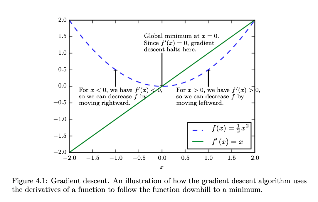
Although the context might be different when dealing with non-convex functions, but let’s take a look at the convex function above. Ultimately, we want to find $x^{\ast }=0$ as $x=0$ minimizes our loss function $f(x)=\frac{1}{2}{x}^2$.

As illustrated in the figure, when $x>0$, moving $x$ slightly towards left will decrease $f(x)$. Similarly, when $x<0$, moving $x$ slightly towards right will decrease $f(x)$. In both situation, the strategy can be formulated as moving $x$ by $-ϵ\cdot sign(f^{{}^{\prime }}(x))$ since $f(x-ϵ\cdot sign(f^{{}^{\prime }}(x)))<f(x)$ for a small enough $ϵ$. This simple technique is called gradient descent which was coined back in 1847 by Cauchy.

Intuitively, $f^{\prime }(x)$ tells us the slope of the function at a certain $x$. For a very steep region, the gradient descent will take a larger step and for a flat region, it will take a flat and smooth step. Finally, when $x=x^{\ast }$ ($x=0$ in this case), $f^{\prime }(x)=0$ which we call as critical points or stationary points what we ultimately aim for.

However, not all critical points are the optimal locations for optimization.

Critical Points

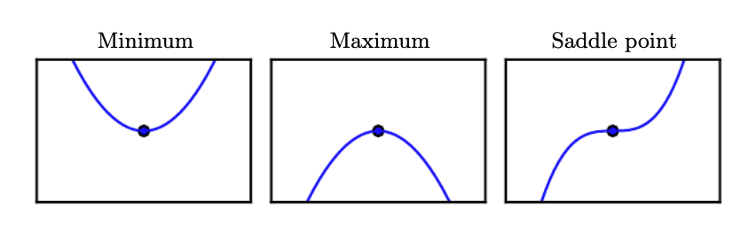
A critical point is a point with zero slope.

deeplearningbook.org

Local Minimum and Maximum points

A local minimum is a critical point which is lower than all the neighboring points and a local maximum is a critical point which is higher than the neighboring points. The gradient descent algorithm will ideally lead us to the local minimum. However, a saddle point might result in a problem.

Saddle points

The third figure in the above shows a saddle point which as neighbors that are both higher and lower the point itself. Different optimization strategies such as SGD have been devised to avoid getting trapped in saddle points.

Global minimum

deeplearningbook.org

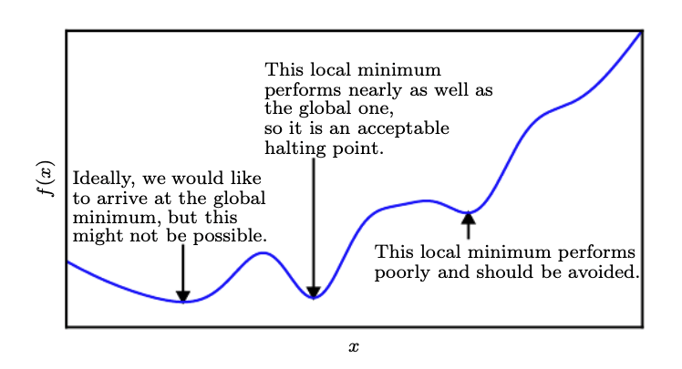
A point that obtains the absolute lowest value of $f(x)$ is a global minimum. There’s only one global minimum for a function. On the other hand, there might be multiple local minima of a function. In the context of deep learning, we typically deal with a loss function that may have many local minima that are not optimal with many saddle points surrouded by very flat regions, making the optimization difficult.

Therefore, we typically aim to settle for a value that is very low although it may not be the global minimum. This optimization is called as approximate minimization as shown in the figure above.

Gradient Descent with multiple inputs - Partial Derivatives

For almost all deep learning tasks, we deal with multiple inputs. Therefore, we must make use of partial derivative.

The partial derivative $\frac{\partial }{\partial x_i}f(x)$ measures how $f$ changes as only $x_i$ increases at point x. The gradient $\mathrm{\nabla }$ generalizes drivative where the derivative is with respect to a vector. Hence, the gradient of $f$ is the vector containing all the partial derivatives, denoted ${\mathrm{\nabla }}_{x}f(x)$

Directional Derivative

The directional derivative in direction $\overrightarrow{u}$ (unit vector) is the slope of $f$ in direction $\overrightarrow{u}$. In other words, it’s the derivative of the function $f(\overrightarrow{x}+\alpha \overrightarrow{u})$ with respect to $\alpha$, evaluated at $\alpha =0$. With chain rule, we can show that,

$$\frac{\partial }{\partial \alpha }f(\overrightarrow{x}+\alpha \overrightarrow{u})={\overrightarrow{u}}^{\mathrm{\top }}{\mathrm{\nabla }}_{x}f(x)$$

when $\alpha =0$.

To minimize $f$, we should find the direction in which $f$ decreases the fastest. This can be done using the directional derivative:

$$\underset{u,u^{\mathrm{\top }}u=1}{min}{u}^{\mathrm{\top }}{\mathrm{\nabla }}_{x}f(x)$$ $$=\underset{u,u^{\mathrm{\top }}u=1}{min}||u|{|}_2||{\mathrm{\nabla }}_{x}f(x)|{|}_2\cos \theta$$

where $\theta$ is the angle between $u$ and the gradient by the dot product formula. Since $||u|{|}_2=1$ and $||{\mathrm{\nabla }}_{x}f(x)|{|}_2$ doesn’t depend on $u$, this simples to

$$mi{n}_u\cos \theta$$

Consequently, this is minimized when $u$ lies in the opposite direction as the gradient ($\theta =\pi$). Now, we can decrease $f$ by moving in the direction of the negative gradient. This method is known as the method of steepest descent or gradient descent.

Gradient Descent Implementation

Learning a theory is great but understanding it with implementation is much better. Let’s implement the gradient descent algorithm for a simple linear regression problem.

Goal

We want to approximate the linear equation $h(x)=\frac{1}{2}x+5$ without the given $\frac{1}{2}$ and $5$. Let’s formulate our equation using $w_0$ and $w_1$.

$$h_w(x)=w_{1}x+w_0$$

Now, our goal is to find $w_0=5$ and $w_1=0.5$ using the gradient descent.

Input and Target Data

We’re given with input data x and the target data y. Remember that our goal is to find $w_0,w_1$ using x and y.

import numpy as np

x = np.array([1.0, 2.0, 3.0, 4.0, 5.0, 6.0, 8.0])
y = np.array([5.5, 6. , 6.5, 7. , 7.5, 8. , 9. ])

Loss Function

We’re using Mean Squared Error (MSE) for linear regression task. Note that $x^{(i)}$ and $y^{(i)}$ denote the $i^{th}$ element in the data.

$$L(w)=\frac{1}{2m}\sum \mathrm{\_}{i=1}^m(h_w(x^{(i)})-y^{(i)}{)}^2$$

def loss_fn(pred, y):
    m = len(pred)
    return (1.0 / (2.0 * m)) * np.sum((pred - y)**2)

Gradient Descent

We’re dealing with linear regression. Our goal is to approximate $w_0$ and $w_1$ as $5$ and $0.5$, respectively. Let’s formulate our problem mathematically.

$$h_w(x)=w_0+w_{1}x$$ $$L(w)=\frac{1}{2m}\sum \mathrm{\_}{i=1}^m(h_w(x^{(i)})-y^{(i)}{)}^2$$ $$\frac{\partial }{\partial w\ast 0}L(w)=\frac{1}{m}\sum \ast {i=1}^m(h_w(x^{(i)})-y^{(i)})$$ $$\frac{\partial }{\partial w\ast 1}L(w)=\frac{1}{m}\sum \ast {i=1}^m(h_w(x^{(i)})-y^{(i)})\cdot x^{(i)}$$

• $h_w(x)$ denotes our linear function we want to approximate
• $L(w)$ is the loss function
• $2m$ is used for $L(x)$ for simpler derivative calculation

Now we calculated the gradients with respect to $w_0$ and $w_1$. Let’s perform the gradient descent. Note that $ϵ$ refers to the learning rate.

$$w_0:=w_0-ϵ\frac{\partial }{\partial w_0}L(w)$$ $$w_1:=w_1-ϵ\frac{\partial }{\partial w_1}L(w)$$

def gradient_descent(x, y, weights, lr=0.01):
    m = len(x)
    pred = weights['w1'] * x + weights['w0']
    loss = loss_fn(pred, y)

    dw0 = (1. / m) * np.sum(pred - y) # Compute partial derivative of loss w.r.t w0
    dw1 = (1. / m) * np.sum((pred - y) * x) # Compute partial derivative of loss w.r.t w1

    weights['w0'] -= lr * dw0 # Update Parameters - gradient descent
    weights['w1'] -= lr * dw1 # Update Parameters - gradient descent

    return loss, weights

Train Function

def train(num_epochs=5000, learning_rate=0.008):
    # Initialize Weights
    weights = {
        "w0": np.random.randn(),
        "w1": np.random.randn(),
    }
    print("[Initial Weights] w0: {}, w1: {}".format(weights['w0'], weights['w1']))
    print("-"*80)

    for epoch in range(num_epochs):
        # Gradient Descent
        loss, weights = gradient_descent(x, y, weights, lr=learning_rate)

        # Show Result for very 500 epochs
        if epoch % 500 == 0 or epoch == num_epochs - 1:
            print("Epoch {}: Loss: {}, w0: {}, w1: {}".format(epoch, loss, weights['w0'], weights['w1']))

Hyperparameters

num_epochs = 5000
learning_rate = 8e-3

Train

train(num_epochs, learning_rate)

[Initial Weights] w0: 0.34099454173956956, w1: -0.5196184029053978
--------------------------------------------------------------------------------
Epoch 0: Loss: 42.04352367497908, w0: 0.4120596524733747, w1: -0.18458753348838164
Epoch 500: Loss: 0.36745533693908383, w0: 3.19570108985647, w1: 0.8409227220614995
Epoch 1000: Loss: 0.06455007700615974, w0: 4.243768803088826, w1: 0.6428900703255838
Epoch 1500: Loss: 0.01133937113612232, w0: 4.683042748645115, w1: 0.5598891504625705
Epoch 2000: Loss: 0.0019919625773713056, w0: 4.867154516242159, w1: 0.5251011867721503
Epoch 2500: Loss: 0.00034992371816885867, w0: 4.944320811467737, w1: 0.5105205963434764
Epoch 3000: Loss: 6.147033580254241e-05, w0: 4.9766633238261795, w1: 0.5044094706926437
Epoch 3500: Loss: 1.079835972094126e-05, w0: 4.990218958479861, w1: 0.501848130196663
Epoch 4000: Loss: 1.8969242829203655e-06, w0: 4.9959004970328165, w1: 0.5007746020921556
Epoch 4500: Loss: 3.3322854841771933e-07, w0: 4.998281785784952, w1: 0.5003246569977878
Epoch 4999: Loss: 5.8741498619485146e-08, w0: 4.999278595714187, w1: 0.500136309516923

Great! We can see that our model correctly approximates $w_0=5$ and $w_1=0.5$ after training!

Full Code

import numpy as np

x = np.array([1.0, 2.0, 3.0, 4.0, 5.0, 6.0, 8.0])
y = np.array([5.5, 6. , 6.5, 7. , 7.5, 8. , 9. ])


def loss_fn(pred, y):
    m = len(pred)
    return (1.0 / (2.0 * m)) * np.sum((pred - y)**2)


def gradient_descent(x, y, weights, lr=0.01):
    m = len(x)
    pred = weights['w1'] * x + weights['w0']
    loss = loss_fn(pred, y)

    dw0 = (1. / m) * np.sum(pred - y) # Compute partial derivative of loss w.r.t w0
    dw1 = (1. / m) * np.sum((pred - y) * x) # Compute partial derivative of loss w.r.t w1

    weights['w0'] -= lr * dw0 # Update Parameters - gradient descent
    weights['w1'] -= lr * dw1 # Update Parameters - gradient descent

    return loss, weights


def train(num_epochs=5000, learning_rate=0.008):
    # Initialize Weights
    weights = {
        "w0": np.random.randn(),
        "w1": np.random.randn(),
    }
    print("[Initial Weights] w0: {}, w1: {}".format(weights['w0'], weights['w1']))
    print("-"*80)

    for epoch in range(num_epochs):
        # Gradient Descent
        loss, weights = gradient_descent(x, y, weights, lr=learning_rate)

        # Show Result for very 500 epochs
        if epoch % 500 == 0 or epoch == num_epochs - 1:
            print("Epoch {}: Loss: {}, w0: {}, w1: {}".format(epoch, loss, weights['w0'], weights['w1']))


num_epochs = 5000
learning_rate = 8e-3
train(num_epochs, learning_rate)

[Initial Weights] w0: -0.63444883580393, w1: -0.5934978392833998
--------------------------------------------------------------------------------
Epoch 0: Loss: 54.63723960560799, w0: -0.5531316024441059, w1: -0.2130507749094102
Epoch 500: Loss: 0.5426904763697837, w0: 2.8072843959994933, w1: 0.9143141517294999
Epoch 1000: Loss: 0.09533325146937867, w0: 4.080972705588344, w1: 0.6736504329178544
Epoch 1500: Loss: 0.01674698420454846, w0: 4.614810435820929, w1: 0.572781662723038
Epoch 2000: Loss: 0.0029419061620646315, w0: 4.838556481124477, w1: 0.5305047925290008
Epoch 2500: Loss: 0.0005167982342781185, w0: 4.93233459000256, w1: 0.512785395832168
Epoch 3000: Loss: 9.078481781538824e-05, w0: 4.971639569417142, w1: 0.505358710321659
Epoch 3500: Loss: 1.5947970792282975e-05, w0: 4.988113365117044, w1: 0.5022459825795308
Epoch 4000: Loss: 2.8015452199158463e-06, w0: 4.995017985060984, w1: 0.5009413529459072
Epoch 4500: Loss: 4.921413339333638e-07, w0: 4.997911900794716, w1: 0.5003945468575067
Epoch 4999: Loss: 8.67546301950183e-08, w0: 4.9991232969074995, w1: 0.5001656532645753