Train and Test set
The central goal in machine learning is that our model must perform well on the previously unseen inputs not the data we trained for. This ability is known as generalization.
The error from the training is called the training error which is for an optimization problem. What separates machine learning from optimization is that we want the generalization error or test error as low as possible.
But how can we affect performance on the test set when we can observe only the training set? The statistical learning theory suggests some answers.
When we sample training set and test set, make sure that the training and test data are generated by a probability distribution over datasets called the data-generating process which make i.i.d assumptions (independent and identically distribution). The data are independent from each other and the training set and test set are identically distributed.
This assumption enables us to describe the data-generating process with a probability distribution over a single example and that distribution is then used to generate very train/test examples. We call this shared underlying distribution as the data-generating distribution, denoted \(p_{data}\).
One immediate consequence of this generating process is that the expected training error of a randomly selected model is equal to the expected test error of that model because both expectations are formed using the same dataset sampling process.
Machine Learning Performance
To evaluate machine learning algorithms, we typically focus on two primary factors,
Make the training error small
Make the gap between the training and test error small
These two factors correspond to the key challenges of machine learning: overfitting and underfitting
Overfitting
Overfitting occurs when the gap between the training error and the test error is too large. In other words, our machine learning algorithm performs much better than on the training set than on the test set.
Underfitting
Underfitting occurs when the model is not able to perform well on the training set.
Capacity
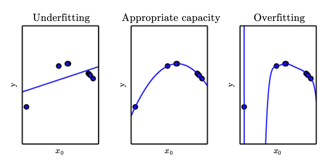
We can control whether our model is more likely to overfit or underfit by changing its capacity. Informally, capacity is its ability to fit a wide variety of functions. A model with a low capacity is likely to underfit on the training set and a model with a high capacity is likely to overfit by memorizing detailed properties of the training set that are not present on the test set.
One way of changing a model’s capacity is changing its hypothesis space.
Changing Hypothesis Space
Hypothesis space is the set of functions that the model is allowed to select as being the solution. For example, in a linear regression algorithm, the hypothesis space is the set of all linear functions of its input. We can modify its hypothesis space to include polynomials, increasing the model’s capacity.
The original linear regression model is
\[\hat{y} = b + wx\]By introducing polynomials \(x^2\), the modified space becomes
\[\hat{y} = b + w_1x + w_2x^2\]Although the increased model is a quadratic function of its input, the output is still a linear function of the parameters. We can keep increasing the capacity of the linear regression model by introducing more higher-order terms.
Machine learning algorithms generally perform best when their capacity is appropriate for the true complexity of the task they need to perform and the amount of training data they are provided with.
To summarize, a model with high capacity can solve complex tasks but if the capacity is too much for a given task or training set, it might result in overfitting. On the other hand, a model with a low capacity cannot solve complex tasks and might result in underfitting. You can see the visualization in the above figure.
Representational Capacity vs Effective Capacity
The model specifies which family of functions the learning algorithm can choose from. This is called the representational capacity of the model. In many situations, finding the exact best solution is a very difficult task. Instead, the learning algorithm will find a function that significantly reduces the training error. This imperfection of the optimization algorithms indicates that the model’s effective capacity may be less than the representational capacity.
Occam’s Razor
This principle (1287-1347) states that among competing hypotheses that explain observations equally well, the simplest one must be chosen. This idea is later formalized in the 20th century by statistical learning theory.
Generalization
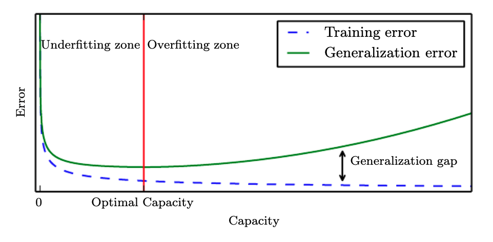
Although simpler functions are more likely to generalize (small gap between training and test error), we must still choose a fairly complex hypothesis to achieve low training error. Typically, training error decreases until it asymptotes to the minimum possible error value as model capacity increases. This is shown in the figure above.
Nonparametric Models
To reach the most extreme case of arbitrarily high capacity, nonparametric models are introduced. While parametric models we have seen so far learn a function described by a parameter vector whose size is finite and fixed before any data is observed, nonparametric models have no such limitation.
Often times, nonparametric models are theoretical abstractions that cannot be implemented in practice but we can design practical nonparametric model by making their complexity a function of the training set size. One example is nearest neighbor regression where the example \((X, y)\) is simply stored and when asked to clasify a test point \(x\), the model looks up in the stored data to find the nearest data point.
Bayes error
The ideal model is one that knows the true probability distribution of the dataset. However, even such a model would still incur some error since there might be noise in the distribution. For supervised learning, the mapping from \(x\) to \(y\) may be inherently stochastic. The error incurred by the ideal model making predictions from the true distribution is called the Bayes error.
Number of training examples
Training and generalization error vary as the size of the training set varies. The expected generalization error can never increase as the training set size increases. For nonparametric models, more data yield better generalization until the lowest possible error is achieved. Any fixed parametric model with less than optimal capacity will asymptote to an error value that exceeds the Bayes error. Also, note that it’s possible for the model to have a large train/test error gap even with the optimal capacity. We can further improve this by introducing more training examples.
The No Free Lunch Theorem
Learning theory claims that a machine learning algorithm can generalize well from a finite training set. However, this doesn’t seem logically correct. You can never perfectly infer general rules from a limited set of examples. To logically infer a rule describing every member of a set, you must have every member of set.
However, machine learning avoids this problem by offering only probabilistic rules: to find rules that are probability correct about most members of the set.
Unfortunately, this still does not solve the entire problem. The no free lunch theorem (Wolpert, 1996) states that averaged over all possible data-generating distributions, every classification model has the same error rate when classifying unseen points. Intuitively, there’s no universally best algorithm. However, in machine learning literature, we make assumptions about the probability distributions we encounter in real-world applications. So, we only design algorithms that perform well on these distributions.
References


