[Paper] AlexNet - ImageNet Classification with Deep Convolutional Neural Networks

The paper for today is ImageNet Classification with Deep Convolutional Neural Networks (AlexNet) by Alex Krizhevsky.

Paper Link: AlexNet

AlexNet

The AlexNet won the first place in ILSVRC-2012\((\)ImageNet Large Scale Visual Recognition Challenge\()\) with 15.3% top-5 test error rate by a considerable margin of 26.2% compared to the second-best model. The AlexNet sparked attention to the effectiveness of CNN.

The author suggests that object recognition task is extremely complex\((\)ex. how many different photos of a dog possible? infinite\()\) which cannot even be all addressed by a large dataset such as ImageNet. Therefore, a more robust model that gives strong and correct insights about nature is needed: CNN. For example, the kernels\((\)filters\()\) in CNN have much smaller size than the entire image dimension and slide through the image with a certain stride. This corresponds to the locality of pixel dependencies of nature.

Dataset

ImageNet dataset consists of over 15 million labeled images with about 22,000 categories which is HUGE. The usual ImageNet that you’ve seen is only a subset with 1000 classes. To maintain a consistent input dimensionality, they’re downsampled to 256 x 256.

Architecture

Krizhevsky et al. 2012

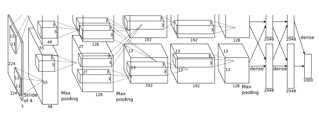
AlexNet has 5 Conv layers and 3 FC layers with ReLU nonlinearity and Local Response Normalization(LRN) which we will see shortly. Also, as we will see in short, data augmentations are performed and the input image dimension is 3x227x227 \((\)The paper says 224x224 but this will lead to wrong dimensions after going through the network\()\). See CS231n.

The ReLU nonlinearity comes right after every conv and FC layer. The author adopted overlapping pooling where the kernel size > stride. It was observed that the overlapping pooling made the model slightly more difficult to overfit.

The reason each layer has two blocks is due to multi-GPU training. Also, it’s funny that the top-portion of the image is cut-off. I assume this is due to the page limit of the journal.

Details of Architecture

The notation is (channels x Height x Width)

Conv Layers

Input: 3 x 227 x 227

Conv1
num_kernels=96, kernel=11, stride=4
Input: 3x227x277
output: 96x55x55

ReLU, LRN

Max Pool
kernel=3, stride=2
Input: 96x55x55
Output: 96x27x27

Conv2
num_kernels=256, kernel=5, stride=1, padding=2
Input: 96x27x27 Output: 256x27x27

ReLU, LRN

Max Pool
kernel=3, stride=2
Input: 256x27x27
Output: 256x13x13

Conv3
num_kernels=384, kernel=3, stride=1, padding=1
Input: 256x13x13
Output: 384x13x13

ReLU

Conv4
num_kernels=384, kernel=3, stride=1, padding=1
Input: 384x13x13
Output: 384x13x13

ReLU

Conv5
num_kernels=256, kernel=3, stride=1, padding=1
Input: 384x13x13
Output: 256x13x13

ReLU

Max Pool
kernel=3, stride=2
Input: 256x13x13 Output: 256x6x6

Classifiers

Dropout

Linear1
Input: 256x6x6
Output: 4096

ReLU, Dropout

Linear2
Input: 4096
Output: 4096

ReLU

Linear3
Input: 4096
Output: 1000

ReLU Nonlinearity

Traditionally, sigmoid \(f(x)=\frac{1}{1+e^{-x}}\) and tanh \(f(x)=\frac{e^x-e^{-x}}{e^x+e^{-x}}\) activation functions were frequently used. However, they have significant disadvantages. If the input values of those functions are too big or small, then the neurons will be saturated \((ex. sigmoid(5) \approx 0.9933)\). Consequently, gradient vanishing could happen. Think about \(g'(x) = g(x)(1-g(x))\) for sigmoid and \(g'(x)=1-g(x)^2\).

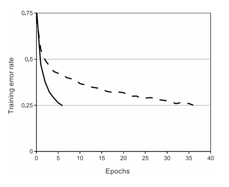
The author adopted ReLU: \(f(x)=max(0,x)\). It was observed that DNN with ReLUs train several times faster than with tanh. Below is the graph comparing training error rate of ReLU\((\)solid line\()\) and tanh\((\)dashed line\()\). As you can see, a 4-layer CNN with ReLUs reach 0.25 error rate approximately 6 times faster than tanh.

ReLU function does not saturate in the positive region and it’s also computationally very efficient. Moreover, it’s actually more biologically plausible than sigmoid and tanh. I’m not an expert in biology, but I guess instead of actually always neurons, it will have to reach some critical point to get activated.

Krizhevsky et al. 2012

Local Response Normalization (LRN)

The author says LRN helps generalization of the network. Let’s look at what it is.

Krizhevsky et al. 2012

• \(a^{i}_{x,y}\): activation computed by applying kernel i at (x,y) and applying ReLU.
• \(b^i_{x,y}\): response-normalized activity
• \(N\): total number of kernels
• \(n\): size of the normalization neighborhood \((\)across channels\()\)
• \(\alpha, \beta, k, n\): hyperparameters

The reason we do \(max(0,i-n/2)\) and \(min(N-1,i+n/2)\) is that we cannot go beyond the ends of our kernel dimension. The sum runs over \(n\) “adjacent” kernal maps at the same spatial position.

The LRN acts like a lateral inhibition in real neurons which compete for big activities amongst neuron outputs computed using different kernels \((\)referenced from paper\()\). Since we normalize accross kernel maps, it resembles brightness normalization. The LRN reduces top-1 and top-5 error rates by 1.4% and 1.2%.

The suggested hyperparameters are \(k=2, n=5, \alpha=10^{-4}, \beta=0.75\)

Data Augmentation

A overfitting-preventing method that is still widely used today is data augmentation. You crop, flip, scale, modify brightness, and so on to give dynamic versatility to the data distribution so that it will better generalize for unseen images. The author in the paper used horizontal flip and random cropping.

During test time, the network extracts 5 cropped images and their horizontal reflections. Then, the network averages the predictions from 10 image patches and give the final prediction.

Also, intensities of the RGB channels are altered for data augmentation by PCA.

Dropout

Another method adopted to prevent overfitting is dropout. What it does is that the network randomly drops certain number of neurons with the probability of 0.5. The effects of dropout is quite interesting. The following are advantages and philosophical intutions behind dropout.

1. It prevents co-adaption of features
   • Since you never know if your close buddies will be removed in next round, you’d hone yourself rather than relying too much on your friend.
2. it performs model-ensembling
   • If you count the combinations of different models from each dropout, it’s A LOT. Probability more than the number of stars in the universe. Each time you perform dropout, you will technically get a different model. Therefore, the final weights are combinations of those different models, in effect.

Weight Initialization

Weights: Gaussian distribution \(N(0,0.01)\)
Biases: 1 for Conv2,4,5, FC1,2,3 and 0 for remaining layers

Learning rate

The learning rate is initially set to 0.01 and gets divided by 10 when the validation error rates stops improving.

Pytorch Code

import torch
import torch.nn as nn

# 1) init function
    # 1-1) Conv layers
    # 1-2) FC layers
    # 1-3) Weight/Bias Initialization
# 2) Forward function

class AlexNet(nn.Module):
    def __init__(self, in_channels=3, num_classes=1000):
        super(AlexNet, self).__init__()

        self.conv_layers = nn.Sequential(
            nn.Conv2d(in_channels, 96, 11, stride=4), # Conv1 / Valid pad
            nn.ReLU(),
            nn.LocalResponseNorm(5, alpha=1e-5, beta=0.75, k=2), # LRN
            nn.MaxPool2d(3, stride=2), # overlapping pool
            nn.Conv2d(96, 256, 5, stride=1, padding=2), # Conv2 / Same pad
            nn.ReLU(),
            nn.LocalResponseNorm(5, alpha=1e-5, beta=0.75, k=2),
            nn.MaxPool2d(3, stride=2),
            nn.Conv2d(256, 384, 3, stride=1, padding=1), # Conv3 / Same pad
            nn.ReLU(),
            nn.Conv2d(384, 384, 3, stride=1, padding=1), # Conv4 / Same pad
            nn.ReLU(),
            nn.Conv2d(384, 256, 3, stride=1, padding=1), # Conv5 / Same pad
            nn.ReLU(),
            nn.MaxPool2d(3, stride=2),
            nn.Flatten()
        )

        self.classifiers = nn.Sequential(
            nn.Dropout(p=0.5),
            nn.Linear(256 * 6 * 6, 4096),
            nn.ReLU(),
            nn.Dropout(p=0.5),
            nn.Linear(4096, 4096),
            nn.ReLU(),
            nn.Linear(4096, num_classes)
        )

        # Initialize Weights/Biases
        self.apply(AlexNet.init_params)

    @staticmethod
    def init_params(m):
        if isinstance(m, nn.Conv2d) or isinstance(m, nn.Linear):
            nn.init.normal_(m.weight, 0, 0.001)
            nn.init.constant_(m.bias, 1)

            # Conv1 layer has in_channels = 3
            # Conv2 layer has in_channels = 256
            # This is unique. So let's take advantage of that.
            # isinstance() required since nn.Linear has name "in_features".
            if isinstance(m, nn.Conv2d) and (m.in_channels == 3 or m.in_channels == 256):
                nn.init.constant_(m.bias, 0)

    def forward(self, x):
        out = self.conv_layers(x)
        out = self.classifiers(out)
        return out # Shape: (batch_size, 1000)