Introduction
Semi-supervised video object segmentation (VOS) is a task that produce the segmentation mask of the subsequent frames given a ground-truth segmentation mask of the initial frame.
Feature matching which compares the extracted features is widely used in VOS task. As VOS requires pixel-wise mask, the feature matching is also generally performed for every single pixel features.
The initial ground-truth frame is called the reference frame and the observing target frame is called the query frame. After the features are extracted from the query frame, they’re compared to those from the reference frame. Then, the simliarity scores are calculated to transfer the reference frame information(label) to the query frame.
The convention VOS methods utilizes surjective matching where the query frame pixels are matched with the best-matching pixels in the reference frame. This approach is robust for large appearance changes but it may cause critical errors when the background distractions exist in the query frame. As there’s no cap of the number of the target pixels in the query frame, the background objects which resemble the target foreground objects may disrupt the prediction.
To overcome this task, the paper proposed a bijective matching algorithm which performs more strictly on prediction than surjective matching. In bijective matching, pixels between the query frame and the reference frame are connected if and only if they’re the bests-matching pixels for each other. Consequently, it exerts a much more strict criteria for matching than surjective matching, resulting in better performance with background distractors.
Also, the mask embedding module is proposed to effectively utilize the position information of a target object. The mask embedding module considers multiple histeoric masks simultaneously to predict future object positions more effectively and accurately. The coordinate information is also fed into the mask embedding module so that the model can perceive the spatial location.
This method achieves comparable performance to other state-of-the-art methods with a much faster inference speed.
The contributions of the paper are as follows
Bijective matching
Mask embedding module
Comparable accuracy with much faster inference speed
Networh Architecture Overview
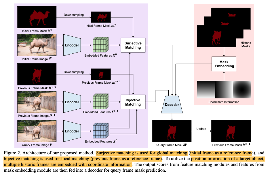
The below figure shows the overall architecture including the bijective matching module and mask embedding module. Next, we’ll jump into each module deeply.
Feature Matching Module
The model utilizes pixel-wise feature matching which means we compare the features of every spatial location to track an object. Let’s formulate terms before delving into the details.
Input image at frame \(i\): \(I^i \in [0,255]^{3 \times H0 \times W0}\)
Extracted features at frame \(i\): \(X^i \in \mathbb{R}^{C \times H \times W}\)
Predicted segmentation mask at frame \(i\): \(M^i \in [0,1]^{2 \times H0 \times W0}\)
Downsampled version of \(M\): \(m^i \in [0,1]^{2 \times H \times W}\)
Initial GT mask of the initial frame: \(M^0\) (0 or 1)
where for \(M, m\), the first channel indicates the background and the second channel indicates the foreground.
Given that the frame \(i\) is a query frame and frame \(k \in [0, i-1]\) is a reference frame, our task is to generate \(M^i\) by using \(X^i, X^k\) and \(m^k\).
The network utilizes both the surjective matching and bijective matching. The surjective matching is used for global matching (initial frame as a reference frame) and the bijective matching is for local matching (previous frame as a reference frame).
Surjective Matching
We first compute the similarity scores between the reference frame and the query frame based on cosine distance between pixels in the feature space. Suppose \(p\) and \(q\) are the single pixel locations in reference frame and the query frame features, then the similarity score is calculated as,
\[sim(p,q) = \frac{\mathcal{N}(X_p^k) \cdot \mathcal{N}(X_q^i) + 1}{2}\]where \(\mathcal{N}\) indicates channel normalization and \(\cdot\) denotes the inner product of matrix.
In order to get the similiarity score between \(0\) and \(1\), we linearly normalize the cosine similarity score. Then, the similairty score matrix
\[S \in [0,1]^{H'W' \times HW}\]is obtained where \(H'W'\) and \(HW\) are the spatial size of reference frame and query frame features, respectively.
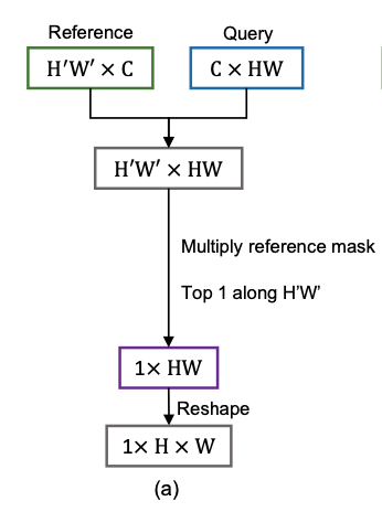
To embody the target object information, the reference frame segmentation mask \(m^k\) is reshaped, expanded for query frame spatial location, and multiplied to the similarity score matrix \(S\) as
\[S\_{BG} = S \odot m_0^k\] \[S\_{FG} = S \odot m_1^k\]where \(\odot\) indicates Hadamard product (element-wise) and \(m_0^k\) and \(m_1^k\) denote the first and second channels of \(m^k\). Finally, we apply query-wise maximum operation to \(S\_{BG}\) and \(S\_{FG}\). In other words, we pick the most similar pixel in the reference frame feature for each pixel in the query frame feature. Consequently, the matching scores
\[Y \in [0,1]^{H \times W}\]are obtained for each class.
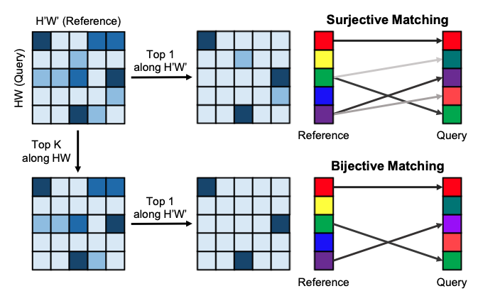
If we observe the above process, it’s definitely surjective which means that only the query frame pixels get to choose the matching partner(specific matching spatial pixel location in a reference frame). By nature, some reference pixels may be referenced multiple times or not referenced at all. This surjective approach is robust against severe variations or rapid apperance change but it may cause critical errors when there are background distractors.
Bijective matching
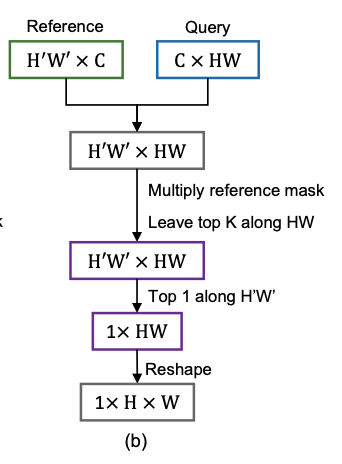
To overcome the drawbacks of surjective matching, the author proposed biject matching. Unlike surjective matching, bijective matching performs a reference-wise top \(K\) operation to remove the background distractions. To preserve homogeneity between the connected pixels, only the maximum \(K\) scores along the query frame are preserved and the others are discarded. Then, the similarity scores for the discarded connections are replaced by the lowest value in each reference frame pixel.
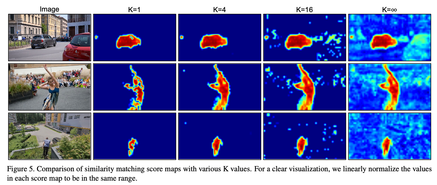
If \(K\) is set to infinity, then no pixel is discarded, being equivalent to the surjective matching. Consequently, query frame pixels can refer to the reference frame pixels if and only if they’re selected at least once by the reference frame pixel. Hence, the bijective matching performs more strictly compared to surjective matching, resulting in safer information transfer.
Surjective vs Bijective matching
The surjective and bijective matching have different advantages complementary to each other.
Surjective matching is effective when the reference frame and the query frame are visually different but susceptible to background distractors. On the other hand, bijective matching is effective for transferring information that are strongly dependent but prone to errors when handling visually different frames because of its strictness.
Integrating the two complementary mechanisms, we feed the matching scores from the two matching methods into the decoder to be used as the appearnce information of a target object.
Mask Embedding Module
The feature matching module is susceptible to visual distractions as it’s completely based on visual information. Therefore, we feed position infomration as well to complement the feature matching module. We observe that the consecutive frames are very related to each other (ex. small changes of objects), we infer that the position of a target object will also be similar in consecutive frames (except when the scene transition happens).
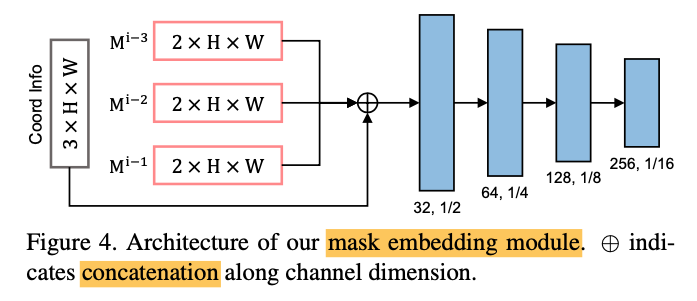
To effectively pass position information, the mask embedding module extracts position information from multiple historic target positions to capture the tendencies of position variation. This was very interesting to me since although it’s a simple method, the network is expected to learn, for example, in what direction the target object is likely to move. We use three historic frames as input
\[M^{i-3} \oplus M^{i-2} \oplus M^{i-1}\]where \(\oplus\) indicates the concatenation along channel dimension. The multiple historic masks simultaneously provides the position-based “coarse” prediction for the current frame’s target location.
In addition, to make the network understand the spatial location, coordinate information is also concatenated along the channel dimension. We use three coordinate information: height, width, and distance from the center point.
Finally, we apply four conv layers with ReLU to embed target position features. The embedded features are fed into the decoder with the outputs from the feature matching module.
The network flow can be found in the “Network Architecture Flow” section above.
Implementation Details
Encoder
For the encoder, the ImageNet pre-trained DenseNet-121 is used to capture obtain rich feature representations. As the original model’s output feature map(before FC layers) is \(1/32\)-sized of the original model, it is difficult to capture the details for the pixel-level classification. Hence, BMVOS uses only first three blocks.
Decoder
As shown in the architecture diagram, the decoder merges high-level features from different modules and refine those features. The outputs from the feature matching module and the output from the mask embedding module are fed into the decoder as input. They’re then gradually refined and upsampled using multi-level features extracted from the encoder using skip connections. This process is essential but naive upsampling high-level features are computationally expensive. Hence, we add channel-reducing deconvolution layers after. every skip connection.
Multi-object processing
We also need to deal with multiple target objects not only a single one. Instead of some previous works which perform for each object one by one, BMVOS shares the image feature embedding which makes the network much more efficient. After predicing the mask for each target object, we aggregate those masks using soft aggregation.
Performances
Different \(K\) values for feature matching module
Quantitative Results
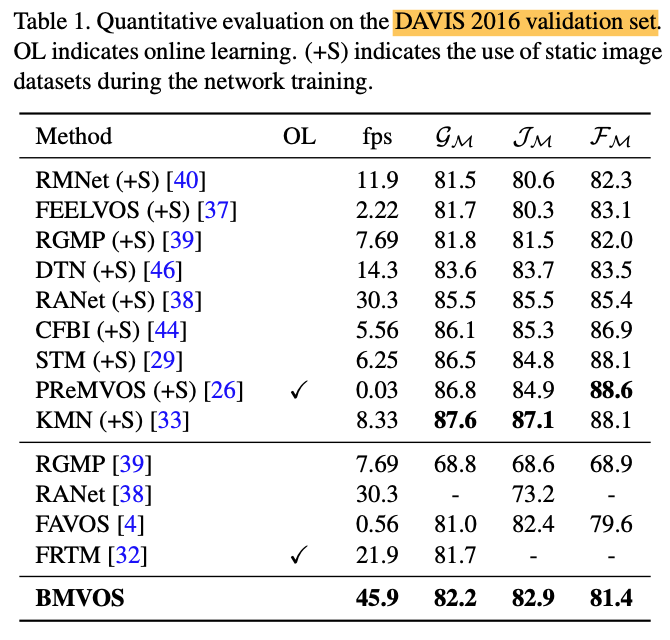
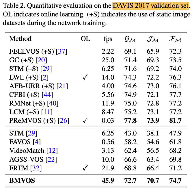
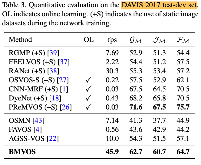
As shown in the tables below, BMVOS shows comparable performances with much faster speed.
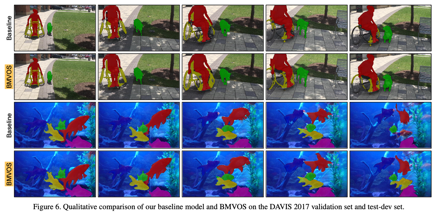
Qualitative Results
References
[1] https://arxiv.org/pdf/2110.01644.pdf

