[Remark] It’s highly recommended to first look at the faster r-cnn paper before studying cascade r-cnn.
Presentation Slides: https://www.slideshare.net/ZGoo/cascade-rcnn-delving-into-high-quality-object-detectionpptx
Introduction
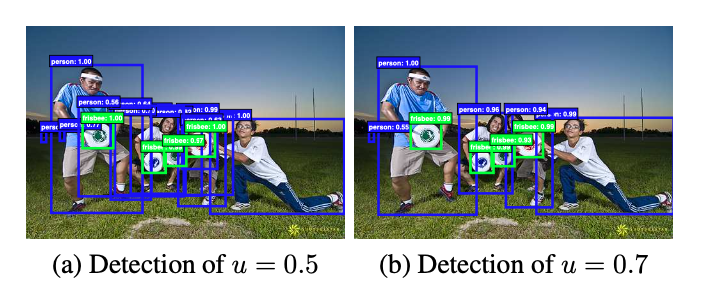
In object detection, there’s a tricky challenge: A detector trained with low IoU threshold (ex. 0.5) usually produces noisy detections and a detector trained with high IoU threshold (ex. 0.7) shows degraded performance.
The paper suggests that there’re two factors for the performance degradation trained with a high IoU threshold,
Overfitting happens during training since the number of positive examples exponentially vanishes if trained with a high IoU threshold (more picky towards the bbox quality)
Mismatch between the IoUs for which the detector is optimal and those of the input hypotheses during inference. In other words, suppose a detector is trained for IoU of
0.7. But for a object detection competition where the criteria ismAP 0.5, then there’s a mismatch between the IoU threshold.
The Cascade R-CNN is proposed to address the above problems. The Cascade R-CNN consists of a sequence of detectors trained with increasing IoU thresholds, to be sequentially more selective against close false positives. The detectors are trained stage by stage, leveraging the observation that the output of a detector is a good distribution for training the next higher quality detector. In other words, suppose a detector is trained with 0.5 IoU threshold, then the output of this will be fed into the next stage detector trained with IoU 0.6 (only 0.1 difference), narrowing the distribution gap between the consecutive stages.
The same procedure is applied at inference as well, enabling a closer match between the hypotheses and the detector quality of each stage.
Background & Cascade R-CNN Motivation
Object detection is a complex problem, mainly dealing with recognition and localization problem. Both tasks are particularly difficult because the detector faces close but not correct bounding boxes (false positives). Therefore, the detector must find the true positives while suppressing the close false positives.
As stated earlier, a detector trained with a low IoU thershold (typically 0.5) establishes a loose requirement for positives, producing rich and diversified but noisy bounding boxes. But a high IoU threshold brings about overfitting problem. How can we deal with this trade-off?
Before diving in, let’s look at some important terms.
The quality of an hypothesis is defined as its IoU with the ground truth.
The quality of a detector is defined as the IoU threshold \(u\) used to train it.
The main idea of this paper is that a single detector can only be optimal for a single quality level. Therefore, the goal is to optimize for a given IoU threshold rather than false positive rate.
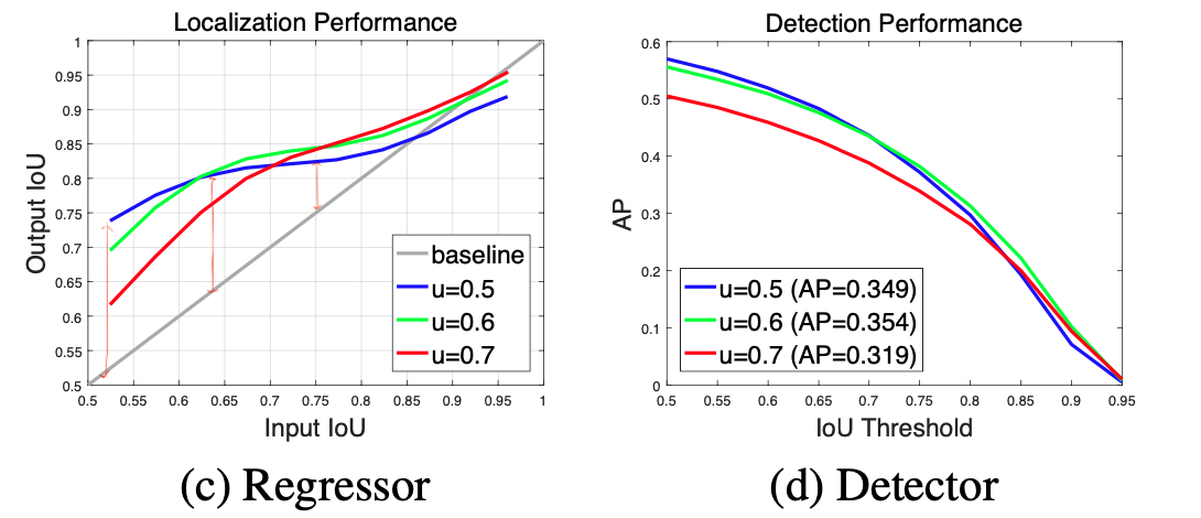
The idea is visualized in the below figure that shows performances of three detectors trained with different IoU thresholds (0.5, 0.6, 0.7)
Localization Performance
The localization performance is evaluated as a function of the IoU of the input proposals. In other words, it’s a graph of quality of output bounding boxes with respect to the proposals by, for example, Region Proposal Network (RPN). Each bounding box regressor performs best for examples of IoU close to the threshold that the detector was trained. For example, if you look at the blue line (\(u\)=0.5), it seems that the vertical gap between the blue line and the gray line decreases as the input IoU increases.
Detection Performance
The phenomenon also holds for detection performance which evaluated as a function of IoU threshold. If you look at the detector of u=0.5, it outperforms the detector of u=0.6 for low IoU levels but underforms at higher IoU levels. In other words, if your detection competition’s criteria is for u=0.5 (low IoU threshold), then the detector of u=0.5 performs better than the the detector of u=0.7 but if the criteria is for u=0.9, then the detector of u=0.5 performs worse than that of u=0.7.
Observations
We can learn some insights from these observations.
A detector optimized at a single IoU level is not necessarily optimal at other levels.
Higher quality detection requires a close match between the detector and the hypotheses that it processes.
A detector can only have high quality if presented with high quality proposals.
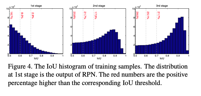
However, just increasing u during training does not resolve the problem. The problem is that the distribution of hypotheses out of a proposal detector is heavily imbalanced towards low quality. So if you increase u, then it will wipe out all those low quality proposals, leaving out only a few positive training samples which inevitably leads to overitting problems.
Also, there’s a mismatch between the quality of the detector and that of the testing hypotheses at inference. High quality detectors are only necessarily optimal for high quality hypotheses. The performance can degrade if they’re asked to work on the hypotheses of other quality levels. For example, the proposals from the RPN are usually not of high quality but rough “guideline” proposals. But if the detector is asked to make really high quality proposals when the proposals it got are garbages (a bit extreme), there comes a quality gap between the two stages, resulting in suboptimal performance. This is like you’re trying to win a battle with bad weapons.
Cascade R-CNN
The Cascade R-CNN is proposed to address these issues. The Cascade-RCNN stages are trained sequentially, using the output of one stage to train the next, making it more selective against close false positives. This is motivated by the observation that the output bounding boxes of a regressor is almost invariably better than the input bounding boxes in terms of IoU with ground truths because that’s why we use the regressor in the first place!
Before diving further, let’s be clear about some notations.
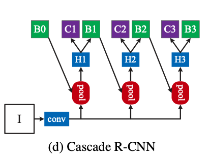
H0: Object proposal sub-network in the 1st stageH1: Region-of-interest detection subnetwork, denoted as detection headC: Classification scoreB: Predicted bounding box locations
(a), (b), (c) show some other architectures. Faster R-CNN produces region proposals through Regional Proposal Network (RPN) and use it’s output as the input of the detection head.
On the other hand, the Cascade R-CNN uses the output of the proposal network as the input of the first detection head. Then, it’s output is again fed into the next stage detection head as input. This process is iterated three times. The intuition is that it’s very difficult to ask a singlw regressor to perform perfectly uniformly at all quality levels. So, the regression task is decomposed into a sequence of simpler steps with sequentially increasing IoU thresholds.
p.s) Personally, the Faster-RCNN diagram in the original Faster-RCNN paper was a bit hard to grasp. In contrast, the diagrams in the Cascade R-CNN paper are very intuitive and simple to understand (even for Faster-RCNN).
Cascaded Bounding Box Regression
The Cascade R-CNN is framed as a cascaded regression problem. The series of cascaded specialized regressors can be formalized as,
\[f(x,b) = f*T \circ f*{T-1} \circ \cdots \circ f_1(x, b)\]where \(T\) is the total number of cascade stages.
Each regressor \(f_t\) is optimized with respect to the sample distribution \(\{b^t\}\) arriving at the corresponding stage, not the initial distribution of \(\{b^1\}\). This procedure improves hypotheses progressively.
The Cascade procedure is different from the iterative BBox architecture in three ways.
The cascaded regression is a resampling procedure that changes the distribution of the hypotheses to be processed by the different stages.
It’s used for both training and inference, so there’s no discrepancy between the training and inference distributions.
The series of specialized regressor are optimized for the resampled distributions of the different stages.
Cascaded Detection
The left in the figure shows that the distribution of the initial hypotheses is heavily tilted towards low quality (e.g. initial output of RPN), inducing ineffective learning for higher quality classifiers. The Cascade R-CNN addresses this problem by resampling mechanism. Startomg frp, a set of examples \((x_i, b_i)\), it resamples an examle distribution \((x'_i, b'_i)\) of higher IoU. In this way, it’s possible to keep the set of positive examples at a roughly constant size even when the IoU threshold increases as illustrated in the Fig 4 as the red dots. As it moves to the next stage, the distribution is tilted more towards high quality examples. There’re two benefits of this process.
There’s no overfitting since we have plentiful examples at each stage.
The detectors of the deeper stages are optimized for higher IoU thresholds. each stage \(t\), the R-CNN has a classifier \(h_t\) and a regressor \(f_t\) optimized for IoU thresold \(u^t\), where \(u^t > u^{t-1}\). This is guaranteed by minimizng the loss,
where
- \[b^t = f_{t-1}(x^{t-1},b^{t-1})\]
- \(g\): ground truth object for \(x^t\)
- \(\lambda=1\): trade-off coefficient
- \([\cdot]\): indicator function (or identity)
Note that the indicator function \([y^t \geq 1]\) is because the label 0 refers to the background class.
Performance
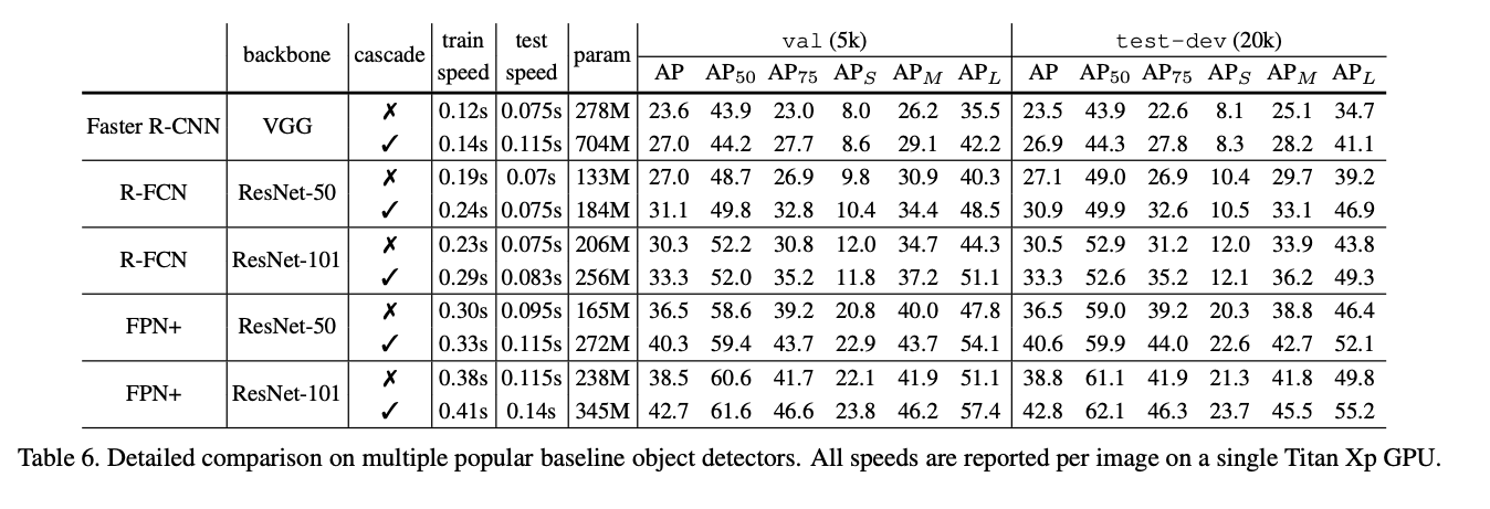
The Cascade R-CNN outperforms all single-model detectors by a marge largin, under all evaluation metrics. The vanilla single-model Cascade R-CNN also surpasses the heavily engineered ensemble detectors that won the COCO challenge in 2015 and 2016. Also, it improves on various baselines consistently by 2~4 points, independently of their strength. These results suggest that the Cascade R-CNN is widely applicable across detector architectures.
References
- https://arxiv.org/abs/1712.00726
- https://deep-learning-study.tistory.com/605

