Reference: https://arxiv.org/pdf/1905.11946.pdf
Presentation slides: slideshare ppt
Intro
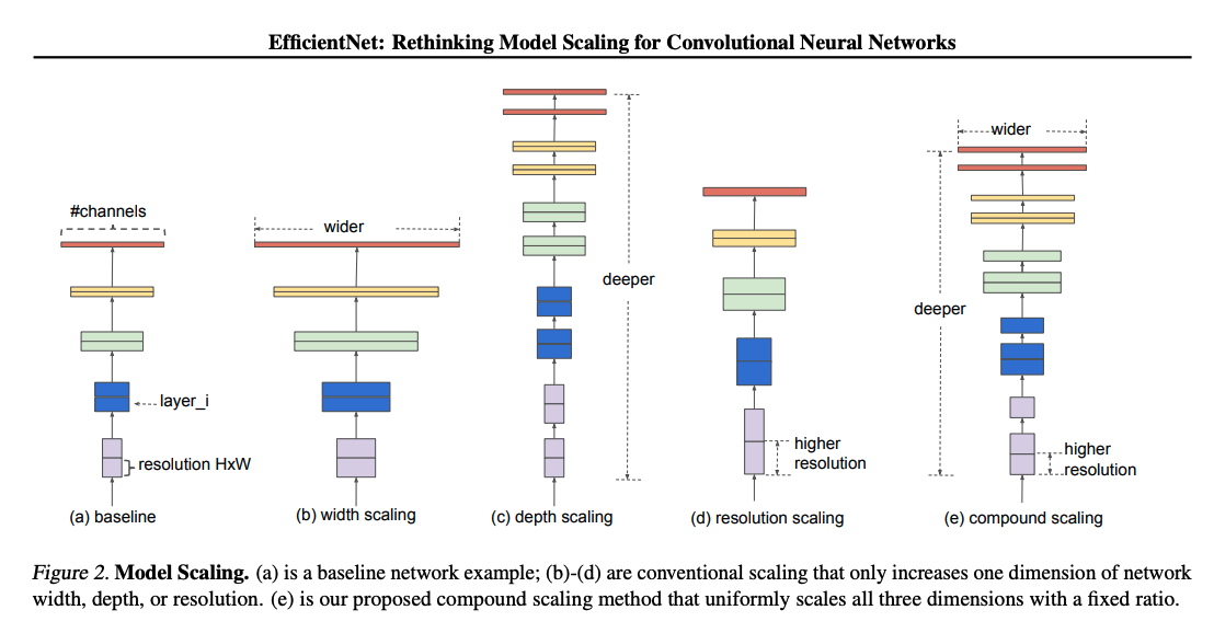
Commonly, ConvNets are designed under a fixed resource budget and scaled up for better accuracy when more resources are available. The most common ways of scaling up are scaling up the network’s depth(more layers), width(more channels), and resolution (spatial dimension).
- Depth Scaling: ResNet
- Width Scaling: Wide ResNet
- Image Resolutin Scaling: GPipe
As above, traditionally, only one of the three dimensions - depth, width, and resolution. Although it’s possible to scale multiple of them, it requires tedious manual tuning with no guarantee of optimal accuracy and efficiency. The author argues that the process of scaling up of CNN has never been fully understood.
The author asks:
Is there a principled way of scaling up network to achieve better accuracy and efficiency?
The empirical studies observe that it’s critical to balance all dimensions of network width/depth/resolution rather than just one. The author proposes that this balancing could be achieved by a simple and effective method called compound scaling method which uniformly scales each with constant ratio.
The compound scaling intuitively makes sense because if you increase the image resolution, more depth(layers) is needed to gain larger effective receptive field and higher width is necessary to capture more fine-grained patterns on the larger image.
Baseline Architecture
Having a baseline architecture is critical. The primary reason is that the network operator \(F_i\), which we’ll see soon, is fixed and we’re manipulating network depth, width and resolution.
A new baseline network is developed using nas(Network Architecture Search) and scaled up using compound scaling method to get a family of models called EfficientNets.
ConvNet Accuracy
Since 2012 with AlexNet, CNN has been increasingly popular. GoogleNet(2015) hit \(74.8\%\) top-1 accuracy with 6.8M parameters. SENet(2018), 2017 ImageNet winner, ahiceved \(82.7\%\) top-1 accuracy with 145M parameters, and GPipe(2018) achieved \(84.3\%\) with 557M parameters.
These networks are so huge that they can only be trained with specialized pipeline parallelism library. Although higer accuracy is important, we’ve already hit the hardware memory limit. Thus, the author suggests,
Let’s take care of efficiency before we further push accuracy
ConvNet Efficiency
Often deep CNNS are overparameterized(too complex w.r.t size of dataset). Model compression is frequently used to reduce the model size, trading efficiency for accuracy such as MobileNets, ShuffleNets, and SqueezeNets. They work out pretty well. Neural Architecture Search(nas) also contribute to better efficiency than hand-crated mobile ConvNets with extensive tunning. However, the way of applying these techniques to very large models is still unclear.
Compound Model Scaling
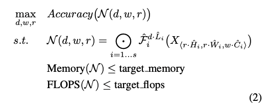
\[Layer\ i:\ Y_i = F_i(X_i)\]1. Formulation
with tensor shape \(<H_i,W_i,C_i>\). \(F_i\) is the operator(ex. kernel op), \(X_i\) is input tensor, and \(Y_i\) is output tensor.
\[ConvNet: \mathcal{N} = \mathcal{F*k} \odot...\odot \mathcal{F_2}\odot \mathcal{F_1}(X_1) = \odot*{j=1...k}\mathcal{F_j}(X_i)\]In practice, ConvNets are often partitioned into stages with same conv operations. Hence, define a ConvNet as:
\[\mathcal{N}=\odot*{j=1...k} F_i^{L_i}(X*{<H_i,W_i,C_i>})\]\(F_i^{L_i}\): Layer \(F_i\) is repeated \(L_i\) times in stage \(i\) \(<H_i,W_i,C_i>\): shape of input tensor X of layer i.
Unlike regular ConvNet designs that look for the best \(F_i\), the paper is trying to expand \(L_i, C_i, H_i, W_i\) with fixed \(F_i\) which is pre-defiend in the baseilne network. Fixing \(F_i\) simplifies the design problem but still enough space to eplore different \(L_i, C_i, H_i, W_i\). For further reducing design space, all layers must be scaled uniformly with constant ratio. Then, the target is treated as an optimization problem that maximizes the model accuracy for a given resource budget.
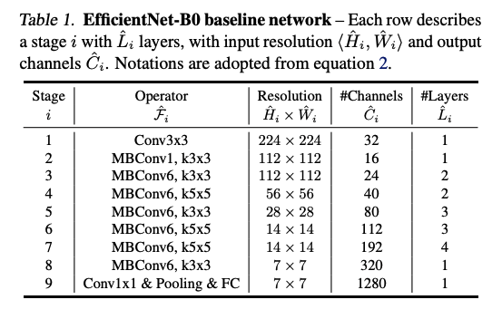
\(w,\ d,\ r\) are coefficients for scaling networth width, depth and resolution. \(\hat{F_i}, \hat{L_i}, \hat{H_i}, \hat{W_i}, \hat{C_i}\) are pre-defined parameters in the baseline network. Below is the EfficientNet-B0 baseline network.
2. Scaling Dimensions
It’s been common to scale only one of the three dimensions - depth, width, and resolution. One of the main reasons is that the otimal \(d,w,r\) are dependent on each other and difference resource budges affect them.
Depth (d)
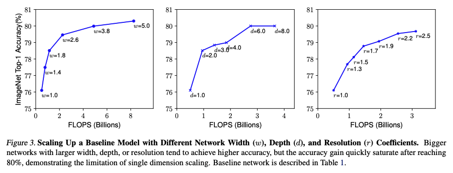
Like ResNet, scaling up network depth is very common and indeed enjoyes higher performance by capturing more complex features. However, deep network suffers gradient vanishing. Although techniques such as shortcut connection and batch normalization are definitely helpful, very deep network still suffers from accuracy saturation. For example, ResNet-1000 shows a similar performance as ResNet-101 despite its huge increase in network depth.
Width (w)
Scaling up network width is also a common method such as Wide-ResNet that is able to capture more fine-grained features. However, very wide networks also show accuracy saturation.
Resolution (r)
Scaling up image resolution can also potentially capture more fine-grained patterns. For example, GPipe(2018) uses \(480*480\) resolution. The resolution scaling contributes to the higher accuracy but very high resolutions also suffer from accuracy saturation.
3. Compound Scaling
We saw that scaling up any dimension improves accuracy but accuracy saturation occurs for larger models.
Also, higher resolution should be balanced with higher depth and width as previously explained. Therefore, we need a way of balancing all the three dimensions rather than a single-dimension scaling.
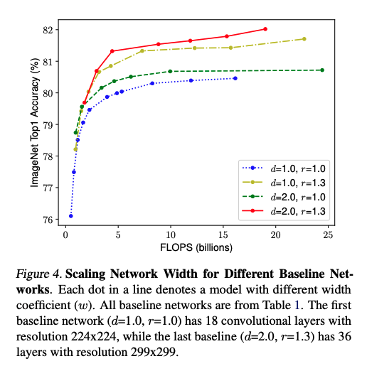
To demonstrate the validity of balanced scaling, the experiment was performed where the accuarcy and FLOPS were recorded with different width scaling under different set of \(d, r\). It’s observed that width scaling with unscaled \(d,r\) quickly saturates. On the otherhand, width scaling under \(d=2, r=1.3\) achieves higher accuracy with similar FLOPs cost.
4. Compound Scaling Method
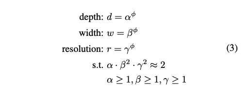
- \(\alpha, \beta, \gamma\) are constant determined by a small grid search. They determine how much to scale depth, width, and resolution, respectively.
- \(\phi\) is a user-defined coefficient that is selected according to the resource budget.
- FLOPs of a regular conv operation is proportional to \(d,w^2,r^2\). If you double the network depth, the FLOPs will be doubled. However, if you double network width, then the FLOPs will be quadrupled since input and output of a layer are both doubled(\(C\) to \(2C\) for input and output, so \(4C^2\)). Doubling resolution obviously increases FLOPs by 4 times.
- Since conv operations usually dominate the CNN computational cost, scaling network dimensions with the method \((3)\) will approximately increase the total FLOPs by \((\alpha * \beta * \gamma)^{\phi}\).
- The paper contraints \(\alpha * \beta^2 * \gamma^2 \approx 2\). Therefore, the total FLOPS will be roughly increased by \(2^\phi\).
EfficientNet Architecture
The above is the EfficientNet-B0 baseline architecture.
- The main buliding block is mobile inverted bottleneck(MBConv)
- Squeeze-and-excitation optimization added.
Starting from this baseline model, we follow the two steps to build EfficientNets family.
- Step 1: Fix \(\phi=1\). Perform a small grid search for \(\alpha,\beta,\gamma\) based on equations \((2), (3)\). The paper foundt the best values for EfficientNet-8 to be \(\alpha=1.2,\beta=1.1,\gamma=1.15\).
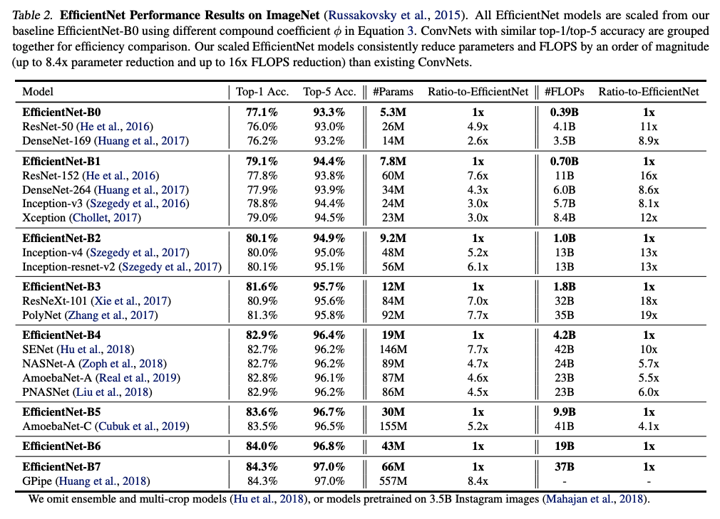
- Step 2: Now fix \(\alpha, \beta, \gamma\) as constants and scale up with different \(\phi\) values based on the equation \((3)\) to obtain EfficientNet-B1 to B7 (Table 2).
Experiments & Performance
1. EfficientNet Performance compared with other models
To demonstrate the effectiveness of the compound model scaling, the Table 2 shows the comparision of number of parameters and FLOPs cost between each EfficientNet model and other models that show similar top-1 and top-5 error to clearly demonstrate the increased efficiency. Taking EfficientNet-B0 as an example, it shows similar top-1 and top-5 accuracy to ResNet-50 and DenseNet-169 but has significantly less parameters \((5.3M)\) and FLOPs \((0.39B)\).
2. Scaling up other models
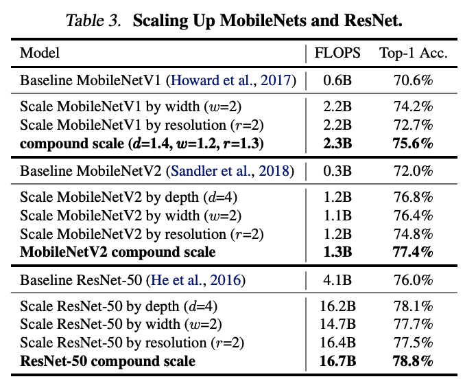
The compound scaling method is applied to ResNet and MobileNets to demonstrate its effect. The compound scaling improves the aaccuracy on these models as shown above. MobileNetV1, MobileNetV2, and ResNet-50 with compound scaling shows \(2.9\%\), \(2.6\%\), and \(0.7\%\) improvement in top-1 accuracy respectively.
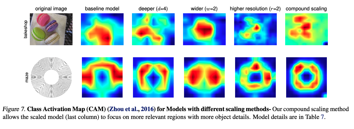
Compound Scaling Activation Map
Compared to single-scaling, compound scaling seems to capture more detailed and generic feature of macarons and maze.

