Introduction
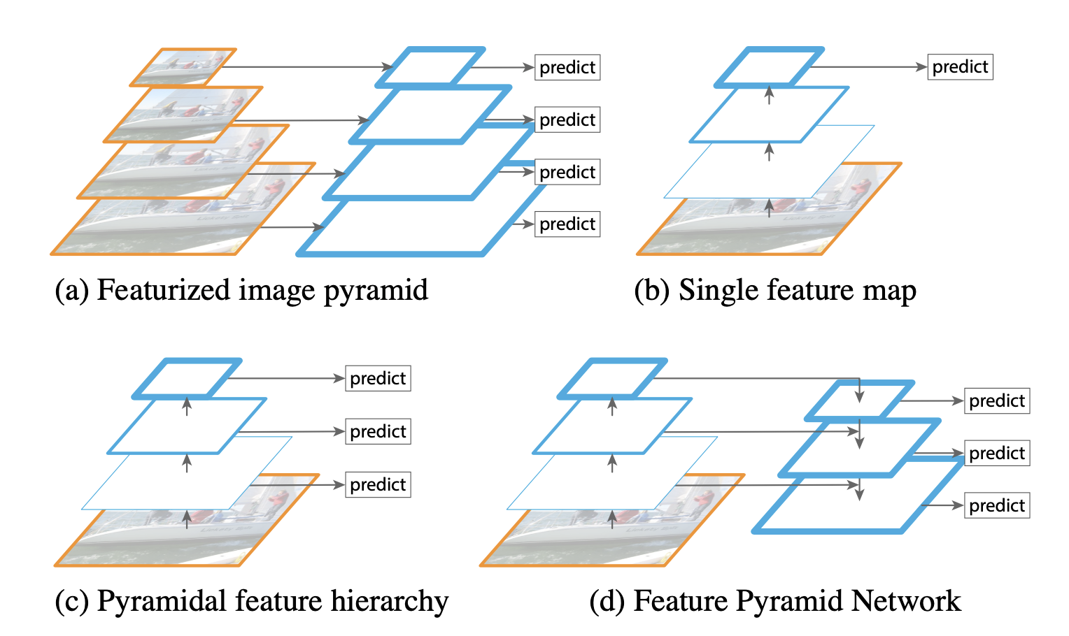
Deep learning based object detection task has been widely studied since the spark of the Convolutional Network (krizhevsky et al. 2012). Algorithms like R-CNN, Fast R-CNN, and Faster R-CNN led to high performance on the detection task. However, recognizing objects with vastly different scales still remained as a fundamental challenge. To address this challenge, different approaches have been made such as Featurized image pyramids where features are computed on each of the image scales independently or Pyramidal feature hierarchy where the pyramidal feature hierarchy of CNN is reused. On the other hand, Feature Pyramid Network (FPN) adopts top-down pathway and lateral connections which we will talk about soon to build more robust and fast pyramid-based detection algorithms. Let’s first look at some common strategies to extract feature maps for detection tasks.
(a) Featurized Image Pyramid
Featurized image pyramid used to be commonly used for detection tasks. An image pyramid is constructed where each differently-scaled image is used to build a feature map. However, this approach considerably increases the inference speed (4x), making this approach impractical for real applications. Also, training deep neural networks end-to-end is also inefficient in terms of memory.
(b) Single Feature Map
Many detection systems use a single scale features for faster detection.
(c) Pyramidal Feature Hierarchy
Each feature map in the pyramidal feature hierarchy of ConvNets are used for detection. However, different feature map levels have large semantic gaps caused by different depths which lead to suboptimal performance.
(d) Feature Pyramid Network (FPN)
FPN (this paper) adopts top-down pathway and lateral connections to shorten the semantic gap between the feature maps of different levels where predictions (e.g, object detection) are independently made on each level.
Feature Pyramid Networks
FPN takes a single-scale image of an arbitrary input size and outputs proportionally sized feature maps at multiple levels. FPN is independent of backbone networks (ResNet is used in the paper). The construction of FPN consists of bottom-up pathway, top-down pathway, and lateral connections.
Bottom-up pathway
The bottom-up pathway is just the feed-forward propagation of the backbone network, spitting out feature maps at different levels with a scaling step of 2. The important thing to note here is that in many ConvNet architectures, there’re many layers producing the same output map size. These layers are considered to be at the same stage just like the stages in ResNet. One pyramid level is constructed for each stage. To be more exact, the last layer of each stage is used as the reference set of feature maps. This choice is from the natural intuition that the deepest layer of each stage should have the strongest features.
For ResNets, the feature-map of the last residual block is used. The output of these last residual blocks are denoted as \(\{C_2, C_3, C_4, C_5\}\) for conv2, conv3, conv4, and conv5 outputs which have strides of \(\{4,8,16,32\}\) with respect to the input image. Conv1 is excluded since it takes too much memory.
Top-down pathway & Lateral connections
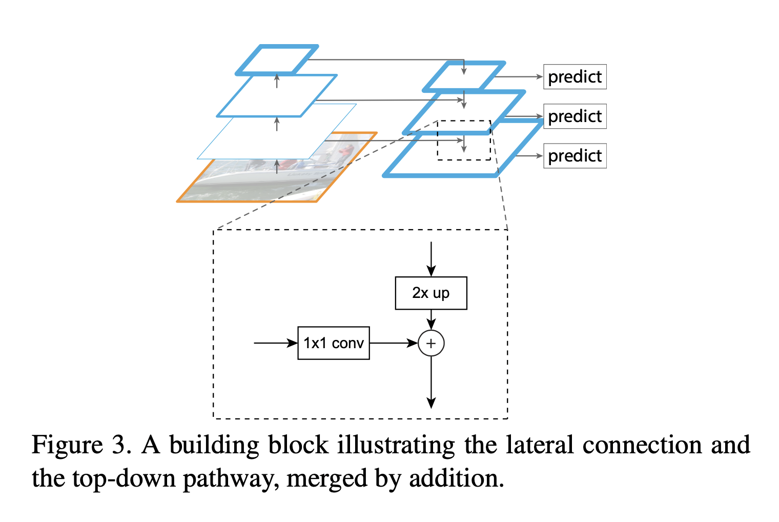
The top-down pathway is the core of FPN. The top-down pathway connects the higher pyramid level feature maps which have spatially coarser but semantically stronger with the feature maps from the bottom-up pathway by upsampling the higher feature maps by a factor of 2 via lateral connections. The lateral connections simply add the feature-maps from the bottom-up pathway (after gone through 1x1 conv) to the upsampled feature-maps from the top-down pathway.
Intuitively, the feature maps from the bottom-up pathway are of lower-level semantics but the activations are more accurately localized. Also, the feature maps from the top-down pathway are of higher-level semantics. By lateral connections, FPN shortens the semantic gaps between levels.
The process is iterated until the finest resolution map is generated. To start this iteration, \(1 \times 1\) convolutional layer is attached to the top feature map (\(C_5\)) obtained from the bottom-up pathway.
\(3 \times 3\) convolution layer is attached to the merged map (via lateral connection) to generate the final feature map. The final set of feature maps is called \(\{P_2, P_3, P_4, P_5\}\), corresponding to \(\{C_2, C_3, C_4, C_5\}\) that are respectively of the same spatial sizes.
Since all levels of the pyramid use shared classifiers/regressors, the feature dimension is fixed (number of channels: \(d\)) in all the feature maps. In the paper, \(d=256\) is used so all extra conv layers have 256-channel outputs.
Lastly, there are no non-linearities in those extra layers as the author found no major impacts.
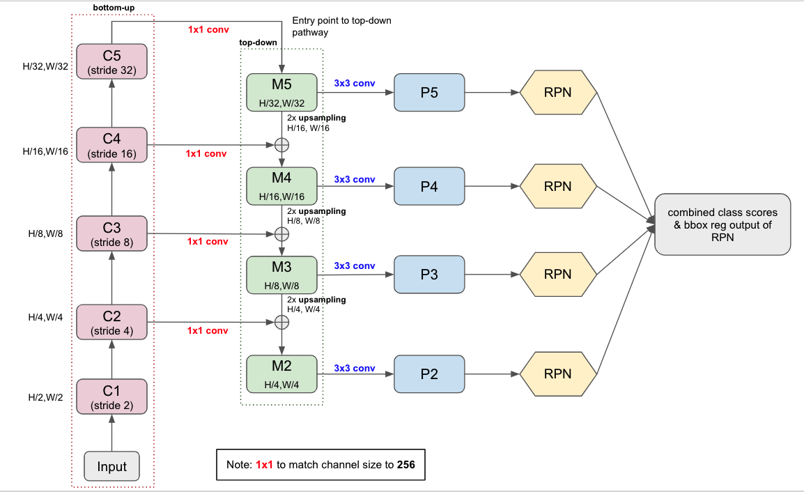
The Figure 3 shows the flow chart of FPN.
- Perform regular feed-forward CNN propagation (bottom-up pathway). For each stage, the spatial dimension is halved.
- After the bottom-up pathway, apply 1x1 convolutional layer to the top feature-map of the bottom-up pathway(\(C_5\)) to obtain the top feature map of the top-down pathway (\(M_5\)) to start the top-down pathway iteration.
- Each top-down feature map is upsampled and merged with the lateral: upsampled \(M_x\) with \(C_{x-1}\)(after 1x1 conv layer)
- Each \(M_x\) goes through \(3 \times 3\) to obtain \(P_x\). Each \(P_x\) is the output of FPN.
- Each \(P_x\) goes through RPN individually and combined later. More implementation details can be found in https://github.com/pytorch/vision/blob/1af20e8c232c7769b3875804e31e3e11cfddef39/torchvision/models/detection/rpn.py for how they’re combined.
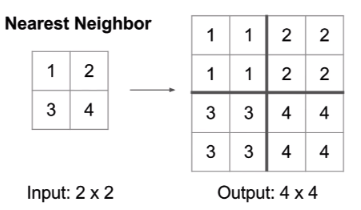
Nearest Neighbor Upsampling
For simplicity, nearest neighbor upsampling is used to match the dimension of top-down pathway.
FPN for RPN
FPN can be applied to any backbone network (ResNet in the paper). Instead of spitting out a single feature map, FPN outputs \(N\) features maps. With these feature maps, RPN is very similarly performed with FPN. The general flow is already shwon in the Figure 3. I’m not going to explain in detail about the Faster-RCNN paper.
One thing to note here is that since the head slides densely over all locations in all pyramid levels, it’s not necessary to have different anchor scales. Instead, anchors of a single scale is assigned to each level. In the paper, the areas of anchors are \(\{32^2,64^2,128^2, 256^2, 512^2\}\) in pixels on \(\{P_2, P_3, P_4, P_5, P_6\}\). The multiple aspect ratios \(\{1:2, 1:1, 2:1\}\) still remain here.
Therefore, we have 15 anchors over the pyramid in total.
FPN for Fast R-CNN
The Fast R-CNN and Faster R-CNN commonly performed on a single-scale feature map. To apply to FPN, we need to assign RoIs of different scales to the pyramid levels. The paper formally defined the assignment strategy:
An RoI of width \(w\) and height \(h\) (on the input image to the network) is assigned to the level \(P_k\) of our feature pyramid by:
\[k = \lfloor k_0 + \log_2(\frac{\sqrt{wh}}{224}) \rfloor\]- \(224\) is the canonical ImageNet pre-training size
- \(k_0\) is the target level on which an RoI with \(w \times h = 224^2\) should be mapped into. \(k_0=4\) in the paper.
The intuitive interpretation is that assigning smaller RoI into smaller feature maps. For example, if the RoI’s scale becomes \(1/2\) of \(224\), then it should be mapped into \(k=3\).
Also note that RoI pooling is applied to extract \(7 \times 7\) features and 2 hidden 1024-d FC layers (each followed by ReLU) are attached before the final classification and bounding box regression layers.
Implementation Details
- The input image is resized so that its shorter side has 800 pixels
- SGD optimizer
- One mini-batch has 2 images per GPU and 256 anchors
- Weight decay of \(0.0001\)
- Momentum of \(0.9\)
- Learning rate is \(0.02\) for the first 30K mini-batches and \(0.002\) for the next 10K
- Unlike the original Faster R-CNN, the anchor boxes outside the image boundary are included for training.
Experiments
Ablation Studies on RPN
The Figure 5 shows the ablation experiments to analyze the impact of FPN. Compared to bottom-up, top-down without lateral connections, and single-scale feature map approach, the FPN shows superior performances for nearly all metrics. In fact, FPN led to dramatic increase of performance.
Ablation Studies on Faster R-CNN
The Figure 5 shows the ablation experiments for Faster R-CNN. Applying FPN to the backbone shows superior performances with considerable increase of AP scores.
PyTorch Implementation
1
2
3
4
5
6
7
8
9
10
11
12
13
14
15
16
17
18
19
20
21
22
23
24
25
26
27
28
29
30
31
32
33
34
35
36
37
38
39
40
41
42
43
44
45
46
47
48
49
50
51
52
53
54
55
56
57
58
59
60
61
62
63
64
65
66
67
68
69
70
71
72
73
74
75
76
77
78
79
80
81
82
83
84
85
86
87
88
89
90
91
92
93
94
95
96
97
98
99
100
101
102
103
import torch
import torch.nn as nn
import torch.nn.functional as F


class FPN(nn.Module):
    def __init__(self,
                 in_channels: list,
                 out_channel,
                 upsample_cfg=dict(mode="nearest")
                ):
        """
        in_channels (List[int]): List of feature map dimensions used for FPN
        out_channel (int): Output dimension(channel) for FPN
        upsample_cfg (dict): config for upsampling (for F.interpolate)
        """
        super().__init__()

        assert type(in_channels) == list
        self.in_channels = in_channels
        self.out_channel = out_channel
        self.upsample_cfg = upsample_cfg # for upsampling
        self.n_in_features = len(in_channels)

        # lateral_conv is 1x1 conv that's applied to bottom-up feature-maps to reduce the channel size
        self.lateral_convs = nn.ModuleList()

        # fpn_conv is 3x3 conv that's applied to P_x
        self.fpn_conv = nn.Conv2d(out_channel, out_channel, kernel_size=3, stride=1, padding=1)

        # Store 1x1 conv layer
        for i in range(self.n_in_features):
            lateral_conv = nn.Conv2d(in_channels[i], out_channel, kernel_size=1, stride=1, padding=0)
            self.lateral_convs.append(lateral_conv)

        self._normal_init(self.lateral_convs, 0, 0.01)
        self._normal_init(self.fpn_conv, 0, 0.01)


    def forward(self, feature_list: list):
        # Construct laterals (after 1x1 conv)
        laterals = [
            self.lateral_convs[idx](feat_map) for (idx, feat_map) in enumerate(feature_list)
        ]

        # Output feature maps of FPN
        outs = []

        # Start Top-down pathway: merge with laterals
        merged = laterals[self.n_in_features - 1] # Start the iteration with top-most
        outs.append(self._copy(self.fpn_conv(merged)))

        # Remaining
        for lateral in laterals[-2::-1]:
            # F.interpolate: Upsampling
            # Lateral connection with element-wise addition
            m = lateral + F.interpolate(merged, size=lateral.shape[-2:], **self.upsample_cfg)
            outs.append(self._copy(self.fpn_conv(m)))
            merged = m

        return outs[::-1]


    def _copy(self, t):
        return t.detach().clone()


    def _normal_init(self, convs, mean, std):
        if isinstance(convs, nn.ModuleList):
            for conv in convs:
                conv.weight.data.normal_(mean, std)
                conv.bias.data.zero_()
        else:
            convs.weight.data.normal_(mean, std)
            convs.bias.data.zero_()


# For Testing
def main():
    in_channels = [2, 3, 5, 7] # Channels
    scales = [340, 170, 84, 43] # Spatial Dimension

    # Creating dummy data
    inputs = [torch.rand(1, c, s, s) for c, s in zip(in_channels, scales)]

    # Output channel
    out_channel = 256

    fpn = FPN(in_channels, out_channel).eval()
    outputs = fpn(inputs)

    for i in range(len(outputs)):
        print(f'outputs[{i}].shape = {outputs[i].shape}')

# Start
main()

'''
outputs[0].shape = torch.Size([1, 256, 340, 340])
outputs[1].shape = torch.Size([1, 256, 170, 170])
outputs[2].shape = torch.Size([1, 256, 84, 84])
outputs[3].shape = torch.Size([1, 256, 43, 43])
'''


