YOLO: You Only Look Once
Paper: https://arxiv.org/pdf/1506.02640.pdf
When YOLOv1 was released in May 2015, it brought many attentions especially due to its extremely high speed. YOLO approached the object detection problem as a regression problem. The best aspect of YOLO is that it’s fully real-time detection algorithm that can process 45 FPS or even 155 FPS with Fast YOLO just in one forward pass in a single network. On the other hand, YOLO is not as accurate as other models and has several downsides as we will cover soon. This post will be a bit long since I want to comprehensively cover everything you need to know about YOLO, make it to the end!
Gentle Introduction
YOLO approaches object detection as a single regression problem. The networks takes RGB images and predict both class probabilities and bounding box locations in one shot through CNN. Consequently YOLO is extremely fast compared to other models such as R-CNN which has complex pipeline including region-proposals. Now, let’s look at some of the advantages of YOLO.
Advantages
1. Extremely Fast
As mentioned many times, YOLO detects objects in one single forwardprop in test time.
2. Global Reasoning
YOLO looks at the entire image and make predictions unlike limited spatial capacity such as sliding window or region proposal-based detections.
3. Good Generalization
YOLO achieves great generalization of objects. YOLO was trained on natural images at first, then tested on artwork images, outperforming DPM and R-CNN by a large gap.
Limitations
Despite its high speed, YOLO(v1) has certain limitations.
1. Low accuracy
YOLO has accuracy-speed trade-off. It does not have state-of-the-art level detection accuracy. YOLO shows a limitation in that it does not precisely localize some objects, especially small ones.
2. Limited Detection Capacity for close-by objects
As we will see later, YOLOv1 can detect only ONE object per one grid cell. This means if two objects belong to the same grid box, it fails to localize both. One way to address this problem is to increase the number of grid cells. We’ll see all of these soon.
YOLO Algorithm
Now, let’s talk about how YOLO actually works.
S x S Grid Cells
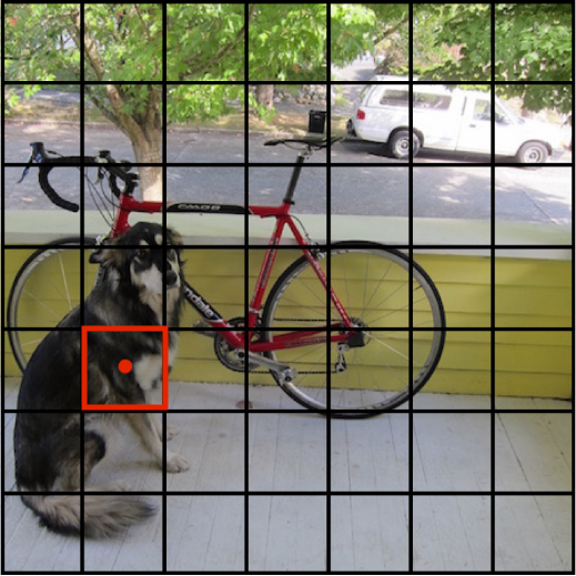
The image box gets divided into S x S grid cells. Each grid cell is responsible for detecting ONE object that also belongs to that grid cell. In other words, YOLOv1 is capable of detecting at most S x S objects.
But how do we know which grid cell the image belongs to? The object belongs to the grid cell that contains the image’s center point. Let’s look at an example.
The dog belongs to the highlighted grid cell since the dog’s center point belongs to the grid cell.
Bounding Box
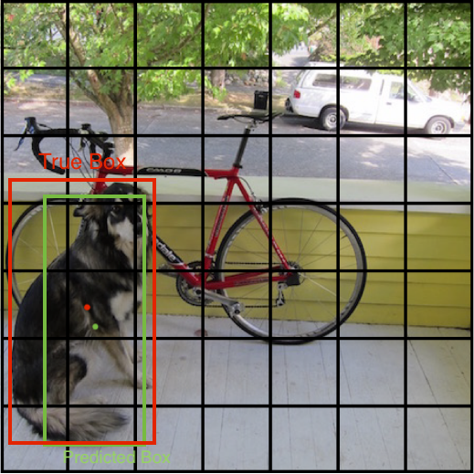
Just like the assignment of an object depends on its center point, the predicted bounding box will have a similar format. Optimally, each grid cell will also draw a bounding box whose center point, hopefully, matches the actual object’s center point. With the center point, the complete bounding box will be formed with width and height. Consequently, each predicted bounding box will have a format of (center x, center y, width, height). Let’s look at an example to get clearer intuition.
The green box is our predicted bounding box. YOLO model predicted that the center point (x,y) of the dog belongs to the grid cell where the green dot is located. Then, YOLO model also predicted that the width and height. The predicted bounding box is in a pretty good shape but slightly off from the actual ground truth bounding box. Yes! that difference will be the key point to our loss function with some other information which we will see soon.
Unfortunately, we’re not done. Although each grid cell can predict only one object, each grid cell is allowed to have multiple bounding boxes. This number of bounding boxes per grid cell is defined by \(B\). This sounds quite contradicting but we have multiple bounding boxes to maximize our capacity to capture various shapes of objects(hopefully vertically-long and horizontally-long?). Later, ONLY ONE of these \(B\) bounding boxes will be selected as the final candidate. We’ll talk about each of them in a minute.
Important Notes
Predicted bounding box will have (x,y,w,h). However, keep in mind that the x and y of the predicted bounding box are relative to each cell and w and h are relative to the whole image.
In the above bounding box, the center point coordinate x and y are always in the range of [0,1]. On the other hand, w and h can be bigger than 1 since it’s relative to the whole image. Of course, if our training images’ bounding boxes are measured differently(for example, x and y are relative to the whole image), then we need to adjust the coordinates accordingly (detailed explanation will be in the codes).
Network Architecture
Now, let’s look at the network architecture for YOLO. After this section, we’ll comprehensively go over what exactly the output of the network represents, how we train our network, and the loss function.
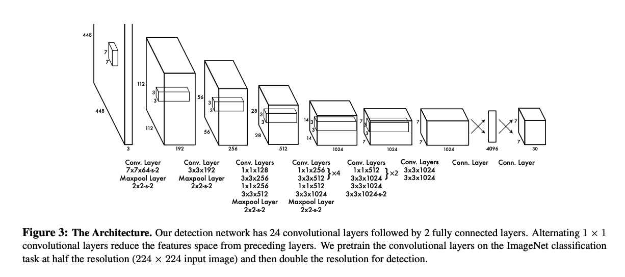
Compared to other complicated computations such as IoU, mAP, Non-max suppression, etc, the network architecture is rather straightforward and simple. The input of the network is 3 x 448 x 448 tensor which represents an RGB image. The model has 24 Conv layers.
Understanding the architecture wouldn’t be hard for you but note that if the padding is not mentioned, always use same padding which preserves the same spatial dimension of the input. The formula for same padding is \(\frac{f-1}{2}\), where \(f\) is the filter(kernel) size.
YOLO used LeakyReLU for nonlinearity.
The most important thing to be aware of is the network’s OUTPUT. As you can in the picture, the output will be 7 x 7 x 30 tensor. Let’s dive into its details.
7 x 7: the paper used \(7\) for $S$ which is the grid size. Also, the paper used \(2\) for \(B\) which is the number of bounding boxes per grid cell. Lastly, the number of classes, \(C\), is assumed to be \(20\) in this summary.30consists ofclass label probabilities,box1 confidence,box1 coordinates,box2 confidence, andbox2 coordinates.output[0:20]: conditional class label probabilities (since there’re 20 classes)output[20]: box1 confidenceoutput[21:25]box1 coordinates \((x,y,w,h)\)output[25]: box2 confidenceoutput[26:30]: box2 coordinates \((x,y,w,h)\)
Therefore, the number 30 comes from the formula \(C + B * 5\), where \(5\) refers to \(confidence, x, y, w, h\). Each box has this list of items, so we do \(B*5\).
Okay, the box coordinates are very straightforward. We can take the maximum class probability as a predicted class label and the \((x,y,w,h)\) is just the coordinate of the predicted bounding box. But, what the heck does the confidence mean?
Confidence Score
When I was first reading the paper, it was a bit confusing to me what this confidence exactly refers to.
The author formally defined confidence as \(Pr(Object) \* IOU^{truth pred}\) where \(Pr(Object)\) denotes the probability that there is an object and \(IOU^{truth pred}\) denotes IoU between the predicted box and the ground truth box. \(Pr(Object)\) is straigtforward but I had hard time understanding how the confidence is determined for the training phase.
My interpretation is that we don’t actually multiply the \(IoU\) but we just define ourselves that the confidence for each box is \(Pr(Object) \* IOU^{truth pred}\), hoping that the predicted confidence (output[20], output[25]) will have value \(1\) when there’s an object in the cell, and \(0\) when there’s no object. In this way, the confidence has two representations.
How confident the model thinks that there is anything in that grid cell
How accurate the model think that the predicted bounding box is
The output also contains conditional class probabilities, denoted as \(Pr(Class_i\|Object)\). This means “If there’s an object, then I’m \(87\%\) positive that it’s a dog”.
If we multiply this conditional class probabilities and confidence score, then we get class-specific confidence score.
\[Pr(Class*i\|Object)\_Pr(Object) * IOU^{truth pred} = Pr(Class_i) \* IOU^{truth pred}\]This class-specific confidence score reflects,
- Probability of that specific class appearing in the grid cell
- How accurate the model think that the predicted bounding box is
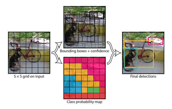
And this is what this picture represents!
In the Bounding boxes + confidence picture, the bold (I assume) predicted boxes are those with higher confidence. Then, in the Class probability map picture, each cell represents class probability and different colors represent different classes.
But how do we get to the final detections? Before we do that, you need to know about IoU and NMS.
Intersection Over Union (IoU)
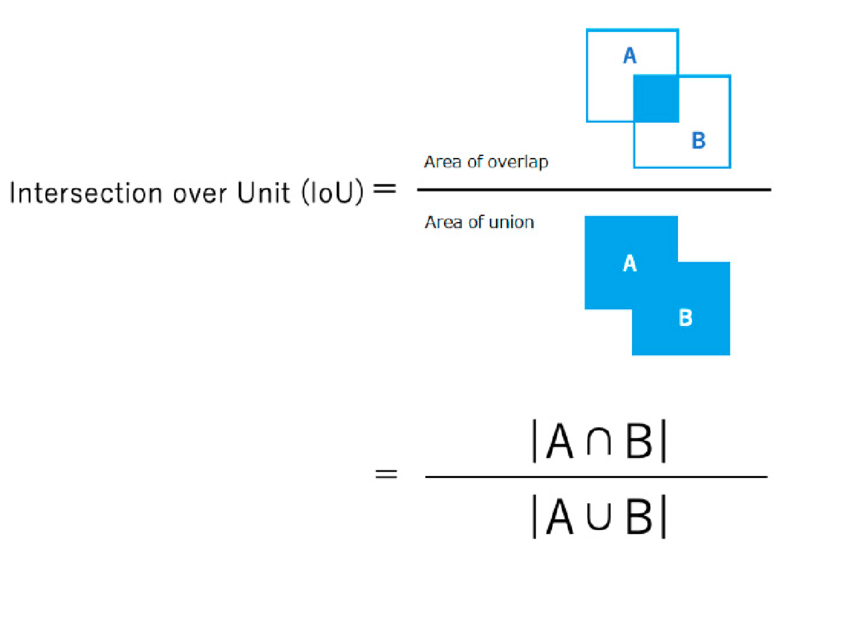
IoU is literally \(\frac{intersection}{union}\). It measures how close two rectangles are. We use IoU to measure how close our predicted bounding box is with the ground truth box. Also, we use IoU for non-max suppression. Let’s look at the diagram.
How do we calculate IoU? Suppose box1(A) has coordinates \((x1,y1,x2,y2)\) and box2(B) has coordinates \((x1',y1'x2',y2')\) where \((x1,y1)\) denotes the upper-left corner and \((x2,y2)\) refers to the bottom-right corner. Then the coordinates for the \(intersection\) will be,
inter_x1= \(max(x1,x1')\)inter_y1= \(max(y1,y1')\)inter_x2= \(min(x2,x2')\)inter_y2= \(min(y2,y2')\)
,assuming that they do overlap. In case they don’t overlap, we just make to \(0\) using .clamp(0) or something else.
The intersection area will be (inter_x2-inter_x1) * (inter_y2-inter_y1).
The union area will be Area of box1 + Area of box2 - intersection area.
NOTE: When the coordinates are given as “midpoint” format, \((x,y,w,h)\), then we must convert it to \((x1,x2,y1,y2)\). Think about it. It’s simple.
That’s it!
Non Max Suppression
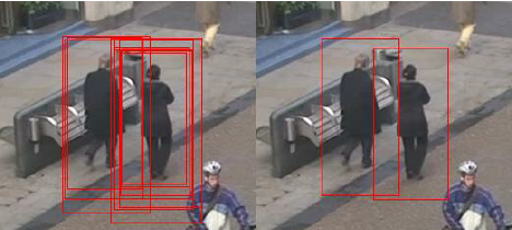
Remember, each grid cell predicts \(B\) bounding boxes and there are \(S*S\) such ones, adding up tot \(B*S\*S\). But surely there are not that may objects. How do we cull out and select the best bounding boxes? That’s why NMS is needed. It’s literally supressing non-max boxes. Here are the procedures of NMS. Note that we’re talking about predictions.
- Before NMS, remove all bounding boxes with
confidence < confidence threshold.- Where this threshold is determined by us. It’s usually
0.5. If the threshold goes up, then it means we’ll grant only the boxes with high confidence, being picky about our performance. If the threshold goes down, then we’re more generous towards not-so-exact predictions.
- Where this threshold is determined by us. It’s usually
For each class, repeat below steps:
Select the bounding box with the highest confidence score.
Loop through the rest of the bounding boxes(same class) and calculate the IoU score between the the one from (2), and the current box. If the
IoU > IoU threshold, then discard that box, removing any redundant bounding boxes.
The result of NMS looks like above.
Forward Pass Prediction
After the image matrix goes through the network, it spits out S x S x 30 output which contains two predicted boxes.
First, we remove all bounding boxes with confidence < confidence threshold.
Second, perform non-max suppression.
Lastly, We select the box with the higher confidence score (B bounding boxes per grid cell might still not be removed) and that is our predicted bounding box for that specific grid cell.
Training: Loss Function
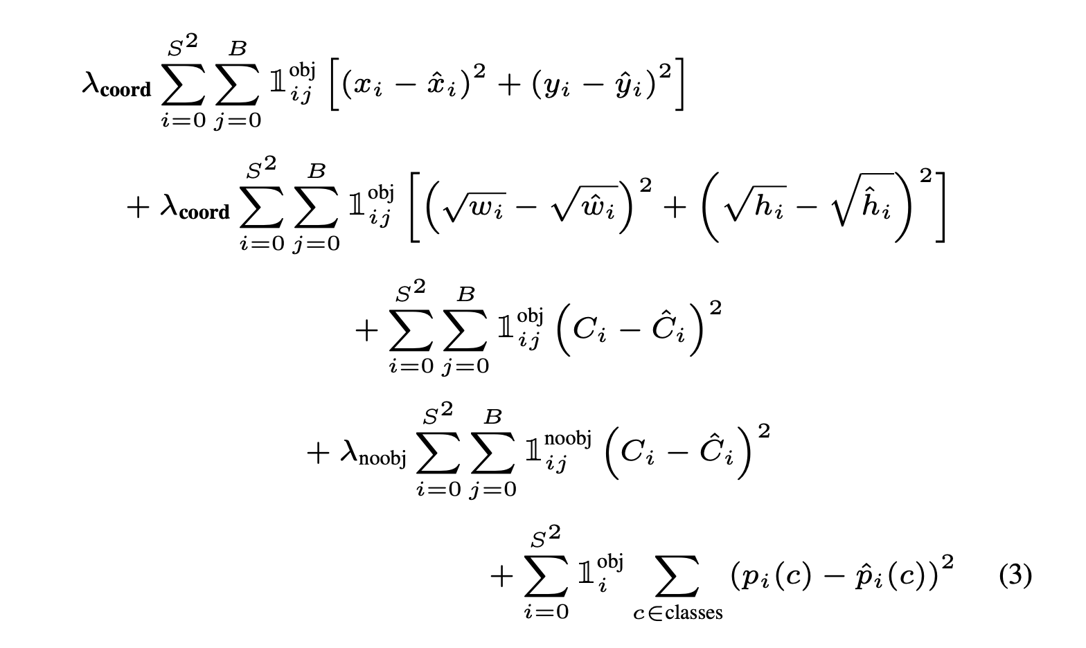
The loss function is divided into three categories,
- \[Coordinate\ Loss\]
- \[Confidence\ Loss\ (Objectness)\]
- \[Class\ Loss\]
Coordinate Loss
Obviously, the predicted bounding’s coordinates \((x,y,w,h)\) will most likely not be the exact same as the ground truth bounding box. Therefore, that coordinate error must contribute to our total loss.
For x and y, we find the Mean Squared Error between our prediction and the ground truth x and y.
Note that \(\lambda*{coord}\) is a parameter that determines “how much the coord loss is amplified”. Since we’re dealing with detection, we put great importance on the coordinate loss. \(\lambda*{coord}=5\) in the paper.
The \(1^{obj}\_{ij}\) denotes the Identity which equals \(1\) if there’s on object in that grid cell and \(0\) if not.
For w and h, we first take square root of those values then find the Mean Squared Error, since w and h are relative to the whole image, so those values will big bigger than x and y. Hence, the author took the square root.
Important: We have two predicted bounding boxes for each grid cell. The one with highest IoU with the ground truth box is “responsible” for the loss.
Confidence Loss (Objectness)
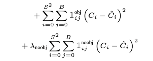
The confidence loss is pretty much the same. We find the MSE of confidence \(\hat{C}\_i\) of the “responsible” predicted bounding box, as stated above, and the that of ground truth.
However, there’s a slight difference. The confidence loss is again divided into two categories.
If there’s an object in the grid cell The above term in the picture corresponds to the confidence loss if there’s indeed an object. \(C_i=1\)
If there’s no object in the grid cell The below term corresponds to this loss. The author took less importance on the noobj loss, so there’s a parameter \(\lambda\_{noobj}=0.5\) to mitigate this no object confidence loss. Also, \(C_i=0\) in this case.
I find it a bit confusing that we still have to choose one responsible box per grid cell. But what if there’s no object? Should we still choose the one with highest IoU or both? I think it makes more sense to penalize both predicted bounding boxes since they both failed.
Class Loss
Notice that the ground truth confidence is \(Pr(Object)\*IoU^{truthpred}\). This is \(1\) when there’s an object since it’s 100% that the object is present and the ideal \(IoU\) must be \(1\) as well. On the other hand, it’s \(0\) when there’s no object for the similar reason.
Finally, we have the class loss. In this case, the identity is \(1^{obj}\_i\). The reason is that each grid cell can have multiple bounding boxes but it always detects only one object. Remember output[0:20] is the class probabilities for both box1 and box2.
For each class, calculate the MSE between the predicted class probabilities and the ground truth class probabilities (which will be one-hot vector).
Evaluation Metric: mAP
Mean Average Precision(mAP) is a frequently used evaluation metric for object detection to determine accuracy. The average precision value is the average of the precision values for recall values which are in the range of \([0,1]\). Let’s first refresh what precision and recall are.
Precision
\[Precision=\frac{TP}{TP+FP}\]The precision tells us how many are true(correct) among those we predicted as true. Therefore, \(TP\)(true positive) denotes the actual number of correct predictions we made while \(FP\)(false positive) refers to the number of “incorrect” predictions while the actual values are “correct”.
Recall
\[Recall=\frac{TP}{TP+FN}\]The recall tells us how many are true among all the correct ground truth values. \(FN\)(false negative) denotes the number of “incorrect” predictions we made while the actual values are “incorrect”. Consequently, recall is always in the range of \([0,1]\) because you obviously cannot make 12 “correct” predictions when there’re only 10 correct values.
Average Precisions
In the object detection problem, \(TP+FN\) is simply the total number of ground truth bounding boxes. This doesn’t change. In otherwords, if we compute the precision and recalls one by one for our predicted bounding boxes, the recall always increses or stays the same. For the precision, we decide that our predicted bounding box is correct if its \(IoU\) with the ground truth is > iou_threshold. In the average-precision graph, x-axis is recall and the y-axis corresponds to precision. Now, we calculate the area under the precision-recall graph. Note that we perform this for each class separately.
Finally, we calculate the average precision with different iou_thresholds. Then, we take the mean of those average precisions to get the mAP.
There’s a great post about more details of mAP: https://jonathan-hui.medium.com/map-mean-average-precision-for-object-detection-45c121a31173
PyTorch Implementation
I hope you guys now have a clearer picture of how YOLOv1 works. However, just passively “understanding” it does not mean you fully understood the algorithm. You MUST implement from scrach to get a comprehensive understanding as well as the subtleties and details. It took me two full days to implement YOLOv1, referencing official github implementation and Youtube. After coding along other people’s codes, I tried implementing everything from scratch on my own. It was painful but I’m sure it helped me a lot. I’ll leave a link below to my implementation with detailed explanations.
With explanation: https://noisrucer.github.io/deeplearning/YOLOv1/
Thanks for reading! Let me know in the comment section what I’ve got to implement next!

