Introduction
YOLO (You Only Look Once) object detection model has been increasingly popular especially due to its extremely fast speed. The original model, YOLOv1, was a breakthrough one-stage model but its performance was not so great despite its extremely fast speed (45 FPS). Joseph Redmon proposed the second version of YOLO model, YOLOv2 which showed various improvements compared to the original model.
There’re two branches of this version: YOLO9000 which can detect over 9000 object categories and YOLOv2 which we will mostly focus on today.
In the following chapters, we’ll talk about the improvements to the original YOLOv2.
Better
Summary
YOLOv1 suffers localization errors and relatively low recall compared to region proposal-based methods. Thus, this paper mostly focuses on improving recall and localization while maintaining classification accuracy.
Many good performing detectors rely on large network or ensembling techniques but YOLOv2 aims for more accurate but still fast detector. Instead of scaling up the network, YOLOv2 simplifies network and make the representation easier to learn.
Batch Normalization
YOLOv2 adopts batch normalization paper link which brings faster convergence and regularization effects. Batch normalization is added on all convolutional layers while dropout layers are removed. It brings more than \(2\%\) mAP improvement.
High Resolution Classifier
YOLOv1 trains the classifier at 224 x 224 scale and increases the reolution to 448 x 448 for detection. This sudden change in resolution makes it hard for the network to adjust to the new input resolution.
YOLOv2 first fine-tunes the classifier at the full 448 x 448 resolution for \(10\) epochs on ImageNet. This gives the network some time to adjust its filters to work better on the higher resolution input.
This method brings almost \(4\%\) mAP increase.
Convolutional With Anchor Boxes
YOLOv2 adopts anchors boxes with which the model predicts the relative coordinates rather than direct predictions of the box coordinates. Predicting the parameterized coordinates simplifies the representation and makes the representation easier to learn.
[1] Shrink the input resolution to
416 x 416
The input resolution is shrunken to 416 x 416 instead of 448 x 448 to have an odd number of locations so that there is a single center cell. The reason we do this is that large objects tend to occupy the center of the image so it’s good to have a single location.
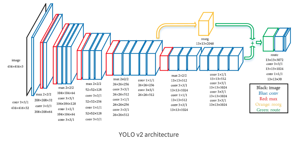
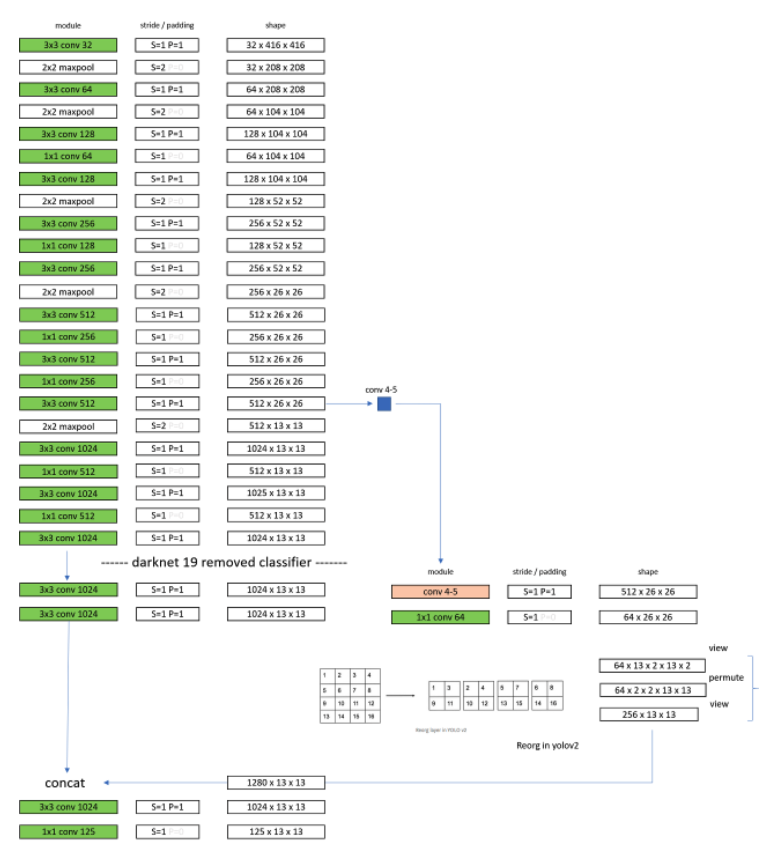
YOLOv2’s convolution layers downsample the input image by a factor of \(32\), so the output feature map will be 13 x 13.
[2] Objectness and class prediction for each anchor box
In YOLOv2, the objectness prediction still predicts the IoU of the GT box and the prediction box. The class prediction predicts the conditional probability of that class given that there’s an object.
The number of output channels is
\[\text{YOLOv1:}\ C+5B\] \[\text{YOLOv2:}\ B(C+5)\]Using anchors boxes bring a small decrease in accuracy. YOLOv1 predicts 98 boxes per image while YOLOv2 predicts more than a thousand.
Without anchor boxes:
69.5 mAP,81% RecallWith anchor boxes:
69.2 mAP,88% Recall
Even though the mAP decreases slightly, the recall increased. This implies that there’s more room to improve.
Dimension Clusters
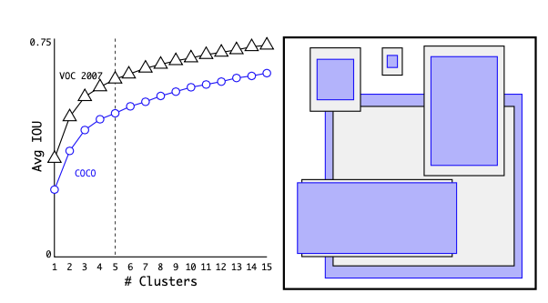
Hand-picked priors (anchor boxes) often lead to suboptimal performances. Instead, YOLOv2 runs k-means clustering on the training set bounding boxes to automatically pick good anchor boxes.
Euclidean distance makes larger boxes more error than smaller boxes so the author proposed to use the distance metric
\[d(box, centroid) = 1 - IOU(box, centroid)\]The author suggested that k=5 is a good tradeoff between the model capacity and high recall.
Relative Location Prediction
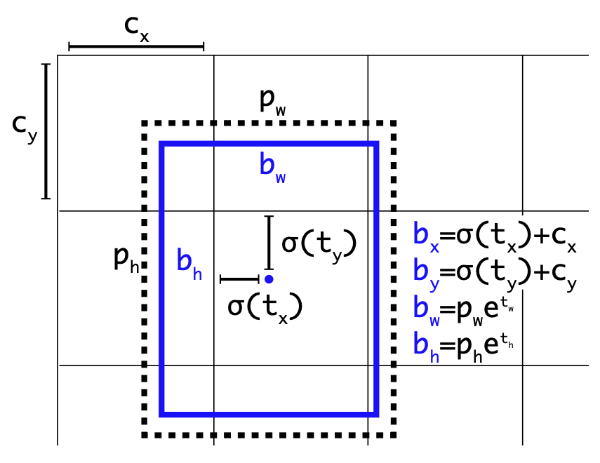
Instead of predicting offsets like in region proposal networks, YOLOv2 predicts location coordinates relative to the location of the grid cell. This bounds the ground truth to fall between 0 and 1. The sigmoid is used to make to fall in [0, 1].
The network predicts 5 coordinates for each bounding box: \(t_x, t_y, t_w, t_h, t_o\). If the cell is offset from the top-left corner of the image by \((c_x, c_y)\) and the anchor box has width and height \(p_w, p_h\), then the predictions correspond to
\(b_x, b_y, b_w, b_h\): Actual bounding box coordinates
\(c_x, c_y\): Top-left corner coordinates of the cell
\(p_w, p_h\): Anchor box width, height
\(\sigma\): logistic activation function: sigmoid
Becuase we constrain the location prediction relative to the cell, the parametrization is easier to learn, making the network more stable.
This prediction method combined with dimension clusters improves YOLO by almost 5% over the region proposal network offset predictions.
Fine-Grained Features
To better capture smaller objects, YOLOv2 adds a passthrough layer which brings features from an earlier layer at 26 x 26 resolution just like the skip-connection from ResNet. The passthrough layer concatenates the higher resolution features (second to last convolutional layer) with the low resolution features by stacking adjacent features into different channels.
During the passthrough connection, 26 x 26 x 512 is turned into 13 x 13 x 2048 which is concatenated with the original features. This gives 1% performances increase.
Multi-Scale Training
YOLOv2 wants to be robust to running on images of different sizes. Instead of fixing the input image size, YOLOv2 changes the network every few iterations.
Every 10 batches, the network randomly chooses a new image dimension size. Since the downsampling factor is 32, the random size is pulled from multiples of \(32\): 320, 352,...,608.
This makes the network to learn a variety of input dimensions.
Faster
YOLOv2 is also fast. The original YOLOv1 uses VGG-16 based feature extractor but it’s needlessly complex with \(30.69\) billion FP operations for a single pass over a single image at \(224 \times 224\) resolution.
YOLOv2 uses a network based on the Googlenet: Darknet-19 for a faster performance.
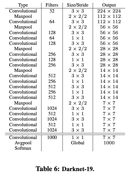
Darknet-19
The author proposed a new classification model Darknet-19 as a backbone of YOLOv2. Similar to VGG, darknet-19 uses 3 x 3 filters and double the channel after every pooling. Also, darknet uses global average pooling to make predictions as well as 1 x 1 comopressing layer between 3x3 convolutions. Batch normalization is used for stabilization, regualrization, and speeding up convergence.
Darknet-19 only has 5.58 billion operations to process an image but achieves 72.9% top-1 accuracy and 91.2% top-5 accuracy on ImageNet.
Training for Classification
First, we train the network on the standard ImageNet 1000 class classification dataset for 160 epochs using SGD with lr=0,1, polynomial rate decay power 4, weight decay 0.0005, momendum-0.9. Standard augmentations such as random crops, rotations, hue, saturation, and exposure shifts are used.
After training on 224 x 224 images, we fine-tune on 448 x 448 resolution for 10 epochs only.
Training for Detection
After tranining the backbone, we remove the last convolutional layer and add three 3 x 3 conv layers with 1024 filters followed by a final 1 x 1 conv layer with the number of outputs for detection.
If we have 20 classes, then the output number of filters would be 5 x (5 + 20) = 125.
Loss Function
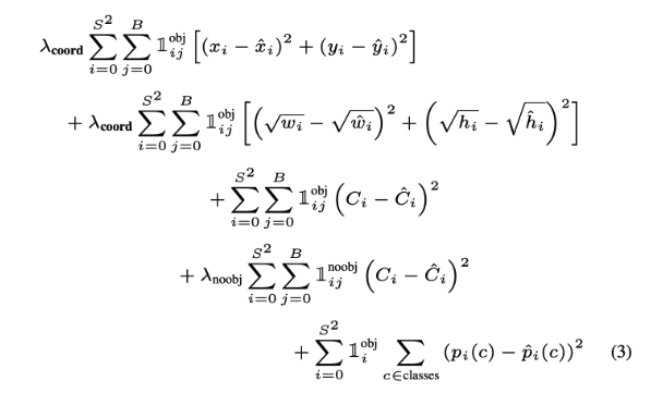
The most annoying part of YOLOv2 paper was that it does not describe its loss function. The above figure shows the YOLOv1 loss function. However, the meanings of some of the variables change. For details about the YOLOv1 loss function, take a look at https://noisrucer.github.io/paper/YOLOv1/
Terms
\(S\):
S x Sgrid\(B\): anchor box
\(\mathbb{1}_{ij}^{obj}\): Indicator function that
cell i, anchor box jhas an object.- \[\lambda_{obj} = 5\]
- \[\lambda_{noobj} = 0.5\]
- \(C_i\): \(1\), GT confidence
YOLOv2 predictions
Then, what does the loss function mean in YOLOv2?
Recall that the predictions of YOLOv2 are \(t_x, t_y, t_w, t_h, t_o\):
\[b_x = \sigma(t_x) + c_x\] \[b_y = \sigma(t_y) + c_y\] \[b_w = p_we^{t_w}\] \[b_h = p_h e^{t_h}\] \[Pr(object) \* IOU(b, object) = \sigma(t_o)\]\(b_x, b_y, b_w, b_h\): Actual bounding box coordinates
\(c_x, c_y\): Top-left corner coordinates of the cell
\(p_w, p_h\): Anchor box width, height
\(\sigma\): logistic activation function: sigmoid
YOLOv2 loss function
In the loss function,
- \(x_i, y_i, w_i, h_i, C_i, p_i(c)\) are the ground truth boxes and those with hats are our predictions.
We can modify the parametrizations little bit to obtain the appropriate ingradients for our loss function
\[b_x - c_x = \sigma(t_x)\] \[b_y - c_y = \sigma(t_y)\] \[\frac{b_w}{p_w} = e^{t_w}\] \[\frac{b_h}{p_h} = e^{t_h}\]So if our model predicts \(t_x, t_y, t_w, t_h\), convert them to \(\sigma(t_x), \sigma(t_y), e^{t_w}, e^{t_h}\) and use as \(\hat{x_i}, \hat{y_i}, \hat{w_i}, \hat{h_i}\).
Then, the ones on the left side of the above equations will be the ground-truth boxes: \(x_i, y_i, w_i, h_i\).
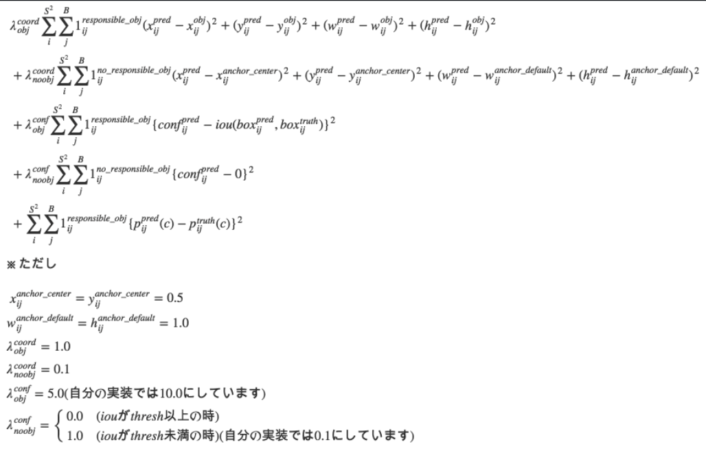
Other suggested loss function
Below is a great suggestion of the loss function of YOLOv2.
Stronger
Hierarchical classification
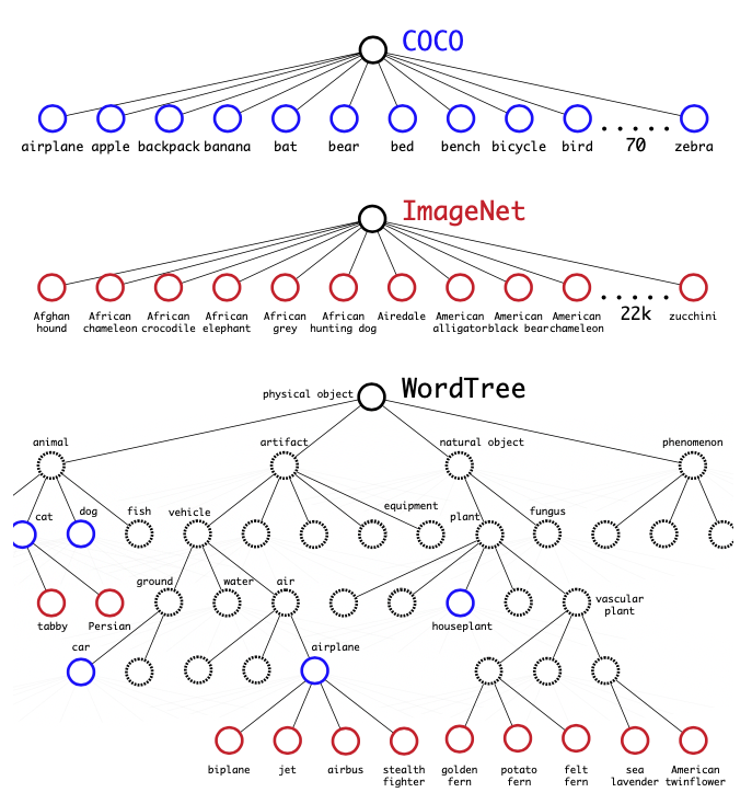
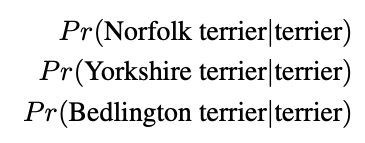
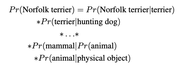
YOLO9000 predicts more than 9000 classes using hierarchical classification. ImageNet labels are pulled from WordNet, a language database that structures how they relate. We merge COCO and ImageNet datasets using the WordNet. Then, we predict conditional probabilities at every node for the probability of each hyponym.
For example, at the -terrior node, we predict
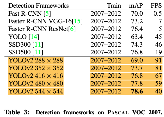
Comparison with YOLOv1
Evaluation
Full PyTorch Implementation
References
[1] https://arxiv.org/abs/1506.02640
[2] https://arxiv.org/abs/1612.08242
[3] https://brunch.co.kr/@kmbmjn95/35
[4] https://wdprogrammer.tistory.com/50

