Introduction
Semantic segmentation is a task to assign each pixel to a desired class label. It’s widely used in fields such as augmented reality devices, autonomous driving, and video surveillance. Two crucial requirements for semantic segmentation task are rich spatial information and sizeable receptive field. Different from some other computer vision tasks including object detection and image classification, semantic segmentation requires very dense prediction for each pixel. Hence, the network architecture must be capable of delivering rich spatial details of the original input image. At the same time, the model must also have enough receptive field to capture the context of the image for accurate predictions. However, modern (as of 2018) approaches compromise sptial resolution for real-time inference speed.
There have been mainly three approaches to boost up the model in the past.
Restricting the input size to reduce the computation complexity by cropping the input image. This approach, however, inherently limits the useful spatial details of the input image which leads to suboptimal performance.
Pruning the network channels to boost up the inference speed, especially in the early stages of the model. However, this approach weakens the spatial capacity.
Dropping the last stage of the model to achive an extremely tight framework. However, this approach has a not enough receptive field to covert large objects.
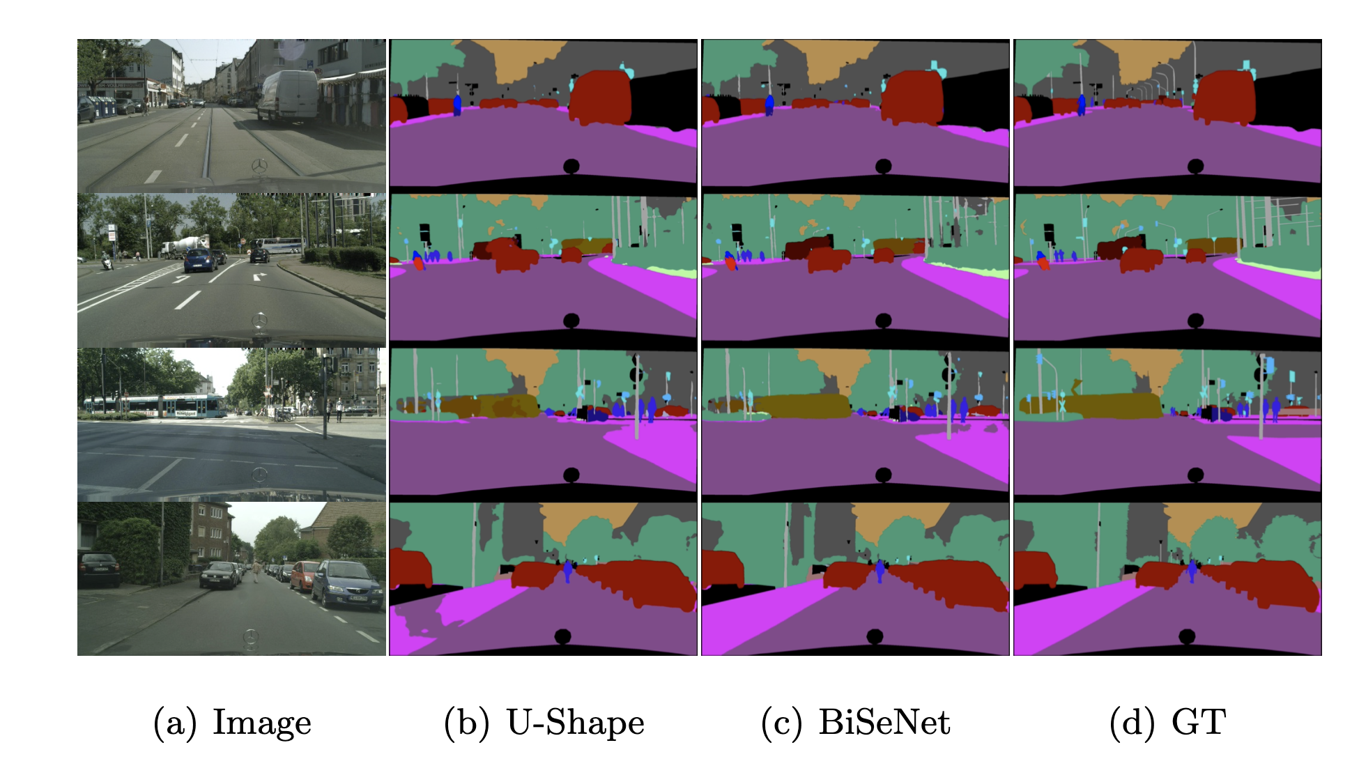
To overcome these weaknesses, a novel U-shape architecture was proposed which gradually increases the spatial resolution, fusing with the hierarchical features of the backbone network. However, this architecture has two drawbacks. First, the complete U-shape architecture reduces the model’s speed due to high-resolution feature maps. Secondly, most spatial information lost in the pruning or cropping cannot be easily recovered.
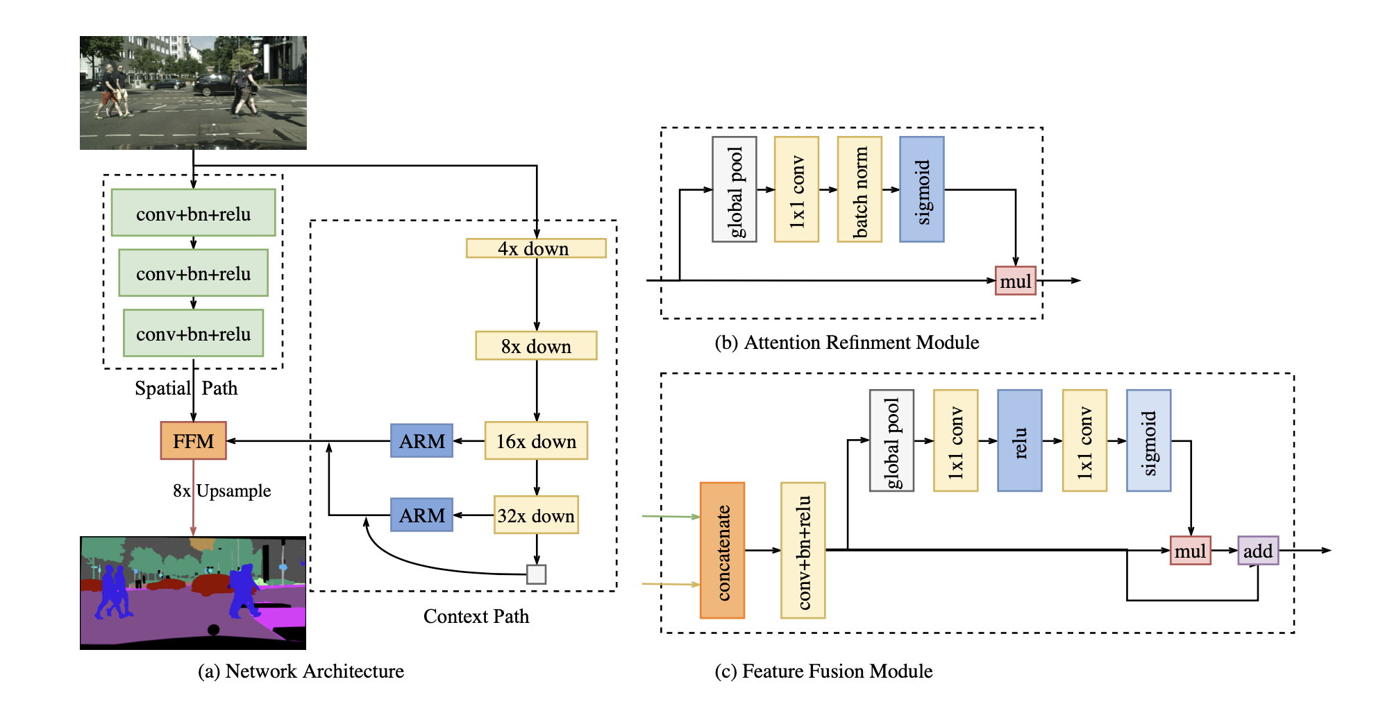
Bilateral Segmentation Network (BiSeNet), 2018 was proposed to challenge this dilemma with simple yet effective methods which we will cover in much detail soon.
BiSeNet Overview
We’ll briefly look at the main components of BiSeNet.
- Spatial Path - rich spatial information
- Context Path - enough receptive field
- Feature Fusion module (FFM) - Fuse spatial path and context path
- Attention Refinement Module (ARM) - refine the features
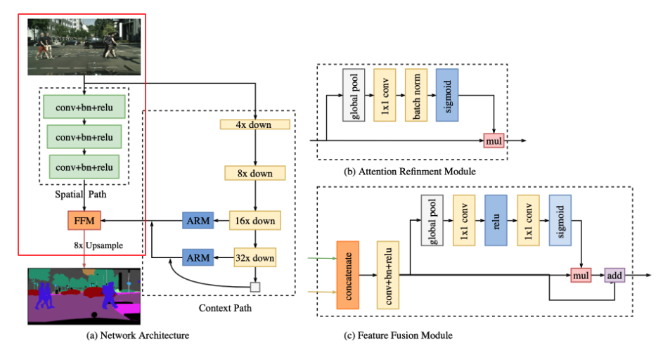
Spatial Path
A few approaches have been proposed to preserve the resolution of the inpute image while some other approaches have been suggested to capture sufficient receptive field such as pyramid pooling, atrous spatial pyramid pooling or, simply large kernel. However, it’s hard to meet the both demands simultaneously. Especially for real-time semantic segmentation, many approaches utilize small input size or lightweight base model to boost up the speed. However, a small input size loses much spatial details of the original image while the lightweight model damages the spatial information with the channel pruning.
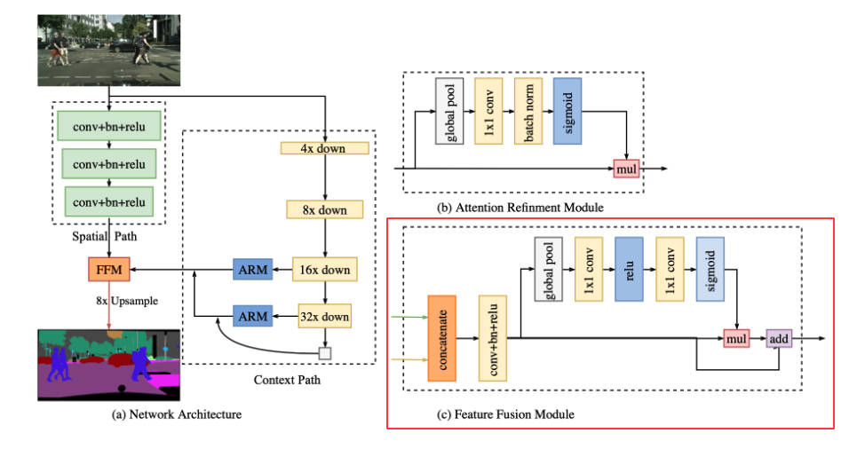
To effectively preserve spatial information, BiSeNet proposes Spatial Path which enables the model to encode affluent spatial information. This module is very simple. It includes three convolution blocks consisting of one convolution layer (stride=2), batch normalization, and ReLU. Finally, Spatial Path downsamples the original image by 1/8 which still contains rich spatial information.
Implementation
1
2
3
4
5
6
7
8
9
10
11
12
13
14
15
16
17
18
19
20
21
22
23
24
25
26
import torch.nn as nn
import torch

class ConvBlock(nn.Sequential):
    def __init__(self, in_channels, out_channels):
        super().__init__(
            nn.Conv2d(in_channels, out_channels, kernel_size=3, stride=2, padding=1),
            nn.BatchNorm2d(out_channels),
            nn.ReLU()
        )


class SpatialPath(nn.Sequential):
    def __init__(self, in_channels=3):
        super().__init__(
            ConvBlock(3, 64),
            ConvBlock(64, 128),
            ConvBlock(128, 256)
        )


if __name__ == '__main__':
    spatial_path = SpatialPath()
    dummy = torch.rand(8, 3, 224, 224) # 1/8 downsample
    assert spatial_path(dummy).shape == torch.Size([8, 256, 28, 28]), "Invalid output shape"
    print("Test Successful")
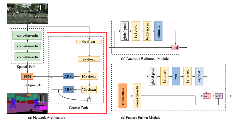
Context Path
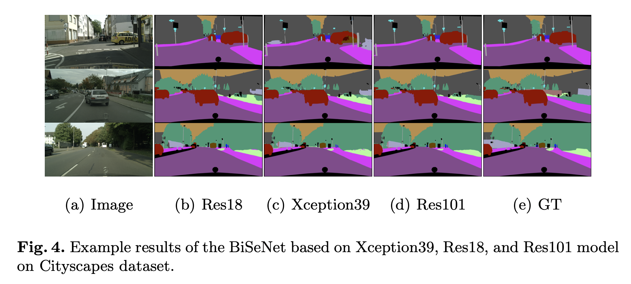
The Spatial Path preserves enough spatial information. Remember that we still need to deal with the receptive field. The Context Path module of BiSeNet was devised to meet this requirement. The Context Path utilizes lightweight model and global average pooling to provide large receptive field. Pre-trained Lightweight models such as Xception, ResNet18 and ResNet101 (bit heavy) were used which quickly downsample the feature map which encodes high-level semantic context information. We also combined the output of the global average pooling, called “tail”, with the features of the lightweight model. The details could be found in the above figure.
Implementation
1
2
3
4
5
6
7
8
9
10
11
12
13
14
15
16
17
18
19
20
21
22
23
24
25
26
27
28
29
30
31
32
33
34
35
36
37
38
39
40
41
42
import torch
import torch.nn as nn
from torchvision import models

class ContextPath(nn.Module):
    def __init__(self, pretrained=True):
        super().__init__()

        resnet18 = models.resnet18(pretrained=pretrained)
        self.conv_block = nn.Sequential( # 1/4
            resnet18.conv1,
            resnet18.bn1,
            resnet18.relu,
            resnet18.maxpool
        )

        self.layer1 = resnet18.layer1 # 1/4
        self.layer2 = resnet18.layer2 # 1/8
        self.layer3 = resnet18.layer3 # 1/16
        self.layer4 = resnet18.layer4 # 1/32

        self.avg_pool = nn.AdaptiveAvgPool2d(output_size=(1, 1))

    def forward(self, x):
        x = self.conv_block(x)
        down_4x = self.layer1(x)
        down_8x = self.layer2(down_4x)
        down_16x = self.layer3(down_8x)
        down_32x = self.layer4(down_16x)
        tail = self.avg_pool(down_32x)

        return down_16x, down_32x, tail


if __name__ == '__main__':
    dummy = torch.randn(8, 3, 224, 224)
    context_path = ContextPath()
    down_16x, down_32x, tail = context_path(dummy)
    assert down_16x.size(2) == dummy.size(2) / 16, "Invalid 16x downsample"
    assert down_32x.size(2) == dummy.size(2) / 32, "Invalid 32x downsample"
    assert tail.size(2) == 1, "Invalid global average pooling"
    print("Test Successful")
Attention Refinement Module
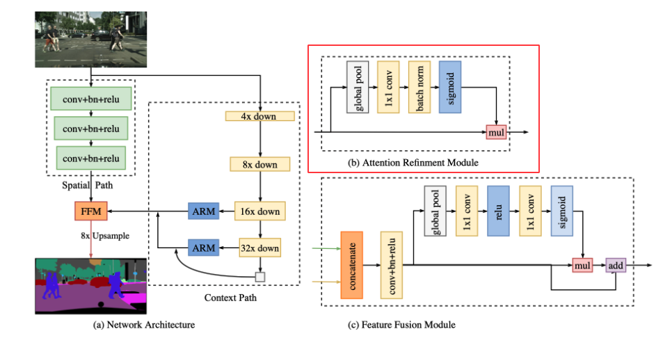
In the Context Path, we attach Attention Refinement Module to 16x and 32x downsampled feature maps from the lightweight model. The ARM module utilizes global average pooling to capture global context and computes an attention vector to guide the feature learning. It integrates the global context information easily without extra up-sampling operation, resulting in negligible computation cost.
Implementation
1
2
3
4
5
6
7
8
9
10
11
12
13
14
15
16
17
18
19
20
21
22
23
24
25
26
27
28
29
30
31
32
33
import torch
import torch.nn as nn

class AttentionRefinementModule(nn.Module):
    def __init__(self, in_channels, out_channels):
        super().__init__()
        assert in_channels == out_channels, "in_channels and out_channels must be the same"
        self.in_channels = in_channels

        self.avg_pool = nn.AdaptiveAvgPool2d(output_size=(1, 1))
        self.conv_1x1 = nn.Conv2d(in_channels, out_channels, kernel_size=1)
        self.batch_norm = nn.BatchNorm2d(out_channels)
        self.sigmoid = nn.Sigmoid()

    def forward(self, x):
        assert x.size(1) == self.in_channels, "in_channels and channel for x must be the same"
        x_copy = x.detach().clone()

        x = self.avg_pool(x)
        x = self.conv_1x1(x)
        x = self.batch_norm(x)
        x = self.sigmoid(x)

        out = torch.mul(x_copy, x)
        return out


if __name__ == '__main__':
    ARM = AttentionRefinementModule(64, 64)
    dummy = torch.randn(8, 64, 224, 224)
    out = ARM(dummy)
    assert out.shape == dummy.shape, "Invalid output shape"
    print("Test Successful")
Feature Fusion Module
The features from the Spatial path and Context Path carry different information in level of feature representation. Therefore, we cannot simply sump up or concatenate them. The feature map from the Spatial Path carry rich and detailed spatial information while the feature map from the Context Path encodes high-level context information. In other words, the Spatial Path is low-level and the Context Path is high-level. To effectively combined these two modules, Feature Fusion Module (FFM) is proposed.
First, we concatenate the two output feature maps from the Spatial Path and the Context Path. Then, we add a convolutional block consisting of a single conv layer, batch normalization, and ReLU. Let’s call the feature at this point fused. Then, we apply the global average pooling and some other modules to compute a weight vector which is multiplied with the copy of fused then added with another copy of fused. The details are shown in the figure above.
Implementation
1
2
3
4
5
6
7
8
9
10
11
12
13
14
15
16
17
18
19
20
21
22
23
24
25
26
27
28
29
30
31
32
33
34
35
36
37
38
39
40
41
42
43
44
45
46
47
48
import torch
import torch.nn as nn


class FeatureFusionModule(nn.Module):
    def __init__(self, in_channels, num_classes):
        super().__init__()
        # in_channels = sum of x1.size(1) + x2.size(2)
        self.in_channels = in_channels

        self.conv_block = nn.Sequential(
            nn.Conv2d(in_channels, num_classes, kernel_size=3, stride=1, padding=1), # same padding
            nn.BatchNorm2d(num_classes),
            nn.ReLU()
        )

        self.avg_pool = nn.AdaptiveAvgPool2d(output_size=(1, 1))
        self.conv_1x1 = nn.Conv2d(num_classes, num_classes, kernel_size=1)
        self.relu = nn.ReLU()
        self.sigmoid = nn.Sigmoid()


    def forward(self, x1, x2):
        x = torch.cat([x1, x2], dim=1)
        assert x.size(1) == self.in_channels, "in_channels and concatenated feature channel must be the same"

        feature = self.conv_block(x)

        attn = self.avg_pool(feature)
        attn = self.conv_1x1(attn)
        attn = self.relu(attn)
        attn = self.conv_1x1(attn)
        attn = self.relu(attn)

        mul = torch.mul(feature, attn)
        add = torch.add(feature, mul)

        return add


if __name__ == '__main__':
    FFM = FeatureFusionModule(64, 10)
    dummy1 = torch.randn(8, 32, 224, 224)
    dummy2 = torch.randn(8, 32, 224, 224)

    out = FFM(dummy1, dummy2)
    assert out.shape == torch.Size([8, 10, 224, 224]), "Invalid output shape"
    print("Test Successful")
BiSeNet Implementation - Combined
Let’s combine all of the 4 modules above to complete the BiSeNet!
1
2
3
4
5
6
7
8
9
10
11
12
13
14
15
16
17
18
19
20
21
22
23
24
25
26
27
28
29
30
31
32
33
34
35
36
37
38
39
40
41
42
43
44
45
46
47
48
49
50
51
52
53
54
55
56
57
58
59
60
61
62
63
64
65
66
67
import torch
import torch.nn as nn

from .spatial_path import SpatialPath
from .context_path import ContextPath
from .attention_refinement_module import AttentionRefinementModule
from .feature_fusion_module import FeatureFusionModule

class BiSeNet(nn.Module):
    def __init__(self, in_channels=3, num_classes=1, training=True):
        super().__init__()
        self.training = training

        self.spatial_path = SpatialPath()
        self.context_path = ContextPath()
        self.attention_refinement_module_16x = AttentionRefinementModule(256, 256)
        self.attention_refinement_module_32x = AttentionRefinementModule(512, 512)
        self.feature_fusion_module = FeatureFusionModule(1024, num_classes) # spatial(256) + context(256+512)
        self.final_conv = nn.Conv2d(num_classes, num_classes, kernel_size=1)

        # Auxiliary Loss Functions
        self.aux_conv_16x = nn.Conv2d(256, num_classes, kernel_size=1)
        self.aux_conv_32x = nn.Conv2d(512, num_classes, kernel_size=1)

    def forward(self, x):
        # Spatial Path
        sp_x = self.spatial_path(x) # 1/8, channel 256

        # Context Path
        # down_16x: 1/16, channel 256
        # down_32x: 1/32, channel 512
        # tail: resolution 1, channel 512
        down_16x, down_32x, tail = self.context_path(x)

        # Attention Refinement Module
        down_16x = self.attention_refinement_module_16x(down_16x)
        down_32x = self.attention_refinement_module_32x(down_32x)
        down_32x = torch.mul(down_32x, tail)

        # Upsampling to match sp_x resolution - 1/8
        down_16x = nn.functional.interpolate(down_16x, size=sp_x.size()[-2:], mode='bilinear', align_corners=True)
        down_32x = nn.functional.interpolate(down_32x, size=sp_x.size()[-2:], mode='bilinear', align_corners=True)

        # For Auxiliary Loss Functions
        if self.training:
            aux_down_16x = self.aux_conv_16x(down_16x) # 1/8, channel num_classes
            aux_down_32x = self.aux_conv_32x(down_32x) # 1/8, channel num_classes
            aux_down_16x = nn.functional.interpolate(aux_down_16x, scale_factor=8, mode='bilinear', align_corners=True)
            aux_down_32x = nn.functional.interpolate(aux_down_32x, scale_factor=8, mode='bilinear', align_corners=True)

        # Concatenate spatial path outputs to feed into Feature Fusion Module
        cp_x = torch.cat([down_16x, down_32x], dim=1) # channel 256+512

        # Feature Fusion Module
        fused = self.feature_fusion_module(sp_x, cp_x) # 1/8, channel num_classes

        # Upsample to original resolution
        fused_upsampled = nn.functional.interpolate(fused, scale_factor=8, mode='bilinear', align_corners=True)

        # Final prediction
        out = self.final_conv(fused_upsampled) # (B, num_classes, H, W)

        if self.training:
            return out, aux_down_16x, aux_down_32x
        else:
            return out
Loss Function
BiSeNet consists of two loss functions: principal loss function and auxiliary loss function.
The principal loss function is used to supervise the output of the whole BiSeNet and the auxiliary loss functions are used to supervise the output of the Context Path.
All loss functions are Softmax Loss.
Also, we use the parameter \(\alpha\) to balance the weight of the losses but the \(\alpha\) used in the paper is \(1\).
\[loss = \frac{1}{N} \sum_i L_i = \frac{1}{N}\sum_i -log \left( \frac{e^{p_i}}{\sum_j e^{p_j}} \right)\]where \(p\) is the output prediction of the network.
\[L(X;W) = l*p(X;W) + \alpha \sum*{i=2}^K l_i(X_i; W)\]where \(l_p\) is the principal loss of the concatenated output. \(X_i\) is the output feature from stage \(i\) of the lightweight model. \(l_i\) is the auxiliary loss for stage \(i\). \(K=3\) in the paper. \(L\) is the joint loss function. We only use the auxiliary function for the training phase.
[Remark] In my implementation, I used binary dice loss and binary cross entropy with balancing weights.
Implementation
1
2
3
4
5
6
7
8
9
10
11
12
13
14
15
16
17
18
19
20
21
22
23
24
25
26
27
28
29
30
31
32
33
34
35
36
37
38
39
40
41
42
43
44
45
46
47
48
49
50
51
52
53
54
import torch
import torch.nn as nn
import torch.nn.functional as F

class BinaryDiceLoss(nn.Module):
    def __init__(self):
        super().__init__()
        self.eps = 1e-5

    def forward(self, pred, target):
        '''
        pred: (B, C, H, W)
        target: (B, H, W)

        Binary Dice Loss
        '''

        pred = pred.squeeze() # (B, H, W)
        pred = torch.sigmoid(pred) # (B, H, W)

        intersection = torch.sum(pred * target, (1, 2))
        cardinality = torch.sum(pred + target, (1, 2))

        dice_score = (2.0 * intersection) / (cardinality + self.eps)
        return torch.mean(1.0 - dice_score)


def binary_dice_loss(pred, target):
    return BinaryDiceLoss()(pred, target)


def bce_with_logits_loss(pred, target):
    #  print(target[0])
    #  print(pred[0])
    pred = pred.squeeze()
    return nn.BCEWithLogitsLoss()(pred, target)


def combined_loss(pred, target, dice_coef=0.25, bce_coef=0.75):
    '''
    pred: (B, 1, H, W)
    target: (B, H, W)
    '''
    dice = binary_dice_loss(pred, target)
    bce = bce_with_logits_loss(pred, target)
    combined = dice_coef * dice + bce_coef * bce
    return combined, dice, bce

if __name__ == '__main__':
    pred = torch.randn(8, 1, 224, 224)
    target = torch.ones(8, 224, 224)
    loss = combined_loss(pred, target, num_classes=2)
    print(loss)
Performances
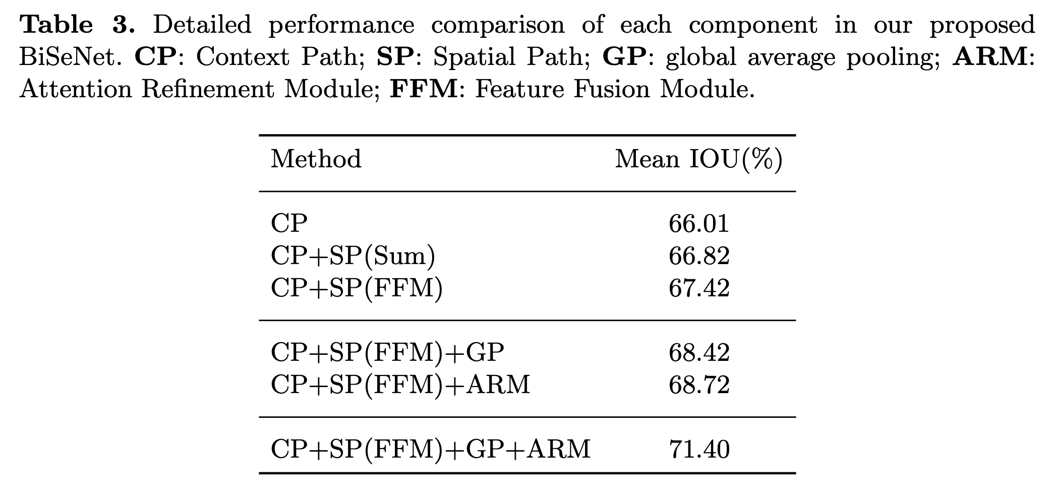
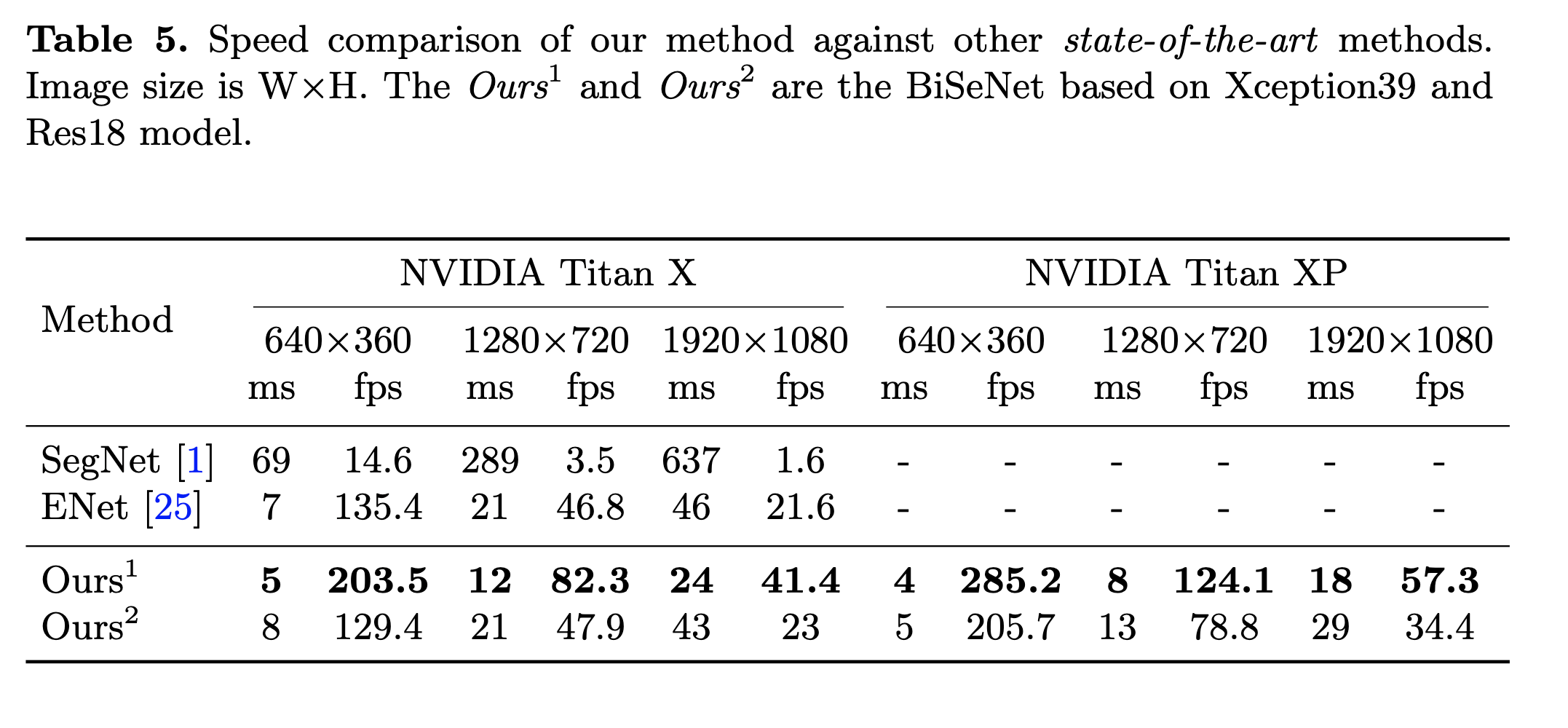
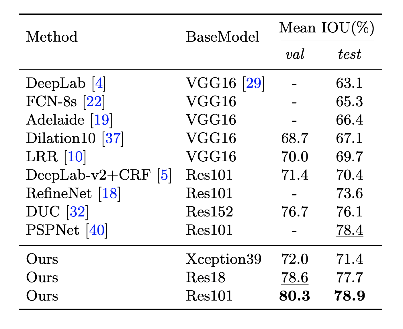
Let’s look at the performance of BiSeNet from various experiments.
GitHub
You can find the full implementation in https://github.com/noisrucer/virtual-background. The project applies BiSeNet for virtual background using webcam.
References
[1] https://arxiv.org/abs/1808.00897
[2] https://github.com/ooooverflow/BiSeNet/blob/master/model/build_BiSeNet.py
[3] https://go-hard.tistory.com/59

