[Paper] U-Net: Convolutional Networks for Biomedical Image Segmentation with Full PyTorch Implementation

Semantic Segmentation

Semantic Segmentation

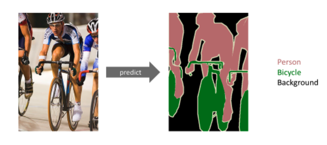
The semantic segmentation task is to label each pixel with a corresponding class.

Introduction

Deep convolutional networks have been dominant in various visual recognition tasks. To adopt convolutional networks for semantic segmentation tasks, it requires precise and dense localization of objects as each pixel is assigned with a corresponding class. The U-Net was first proposed for the biomedical image segmentation where it’s hard to obtain a large number of training images. U-Net exploits heavy data augmentations and effective U-shape architecture for enhanced segmentation performance to train with a small number of dataset.

U-Net Architecture

U-Net

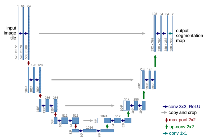
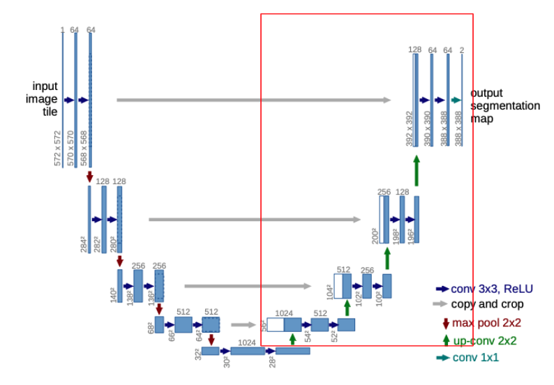
The U-Net architecture consists of a contracting path to capture context and a symmetric expansive or expanding path that enables precise localization.

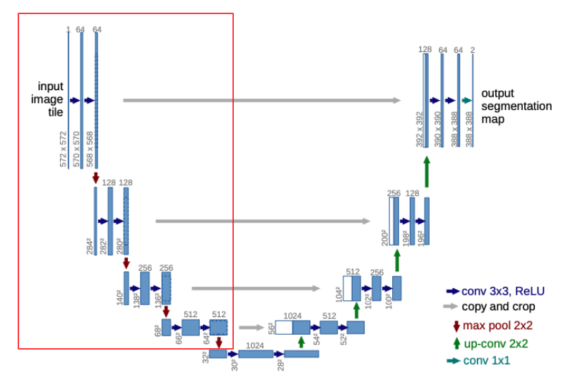
The contracting path is a series of convolutional layers where the channel dimension increases and the spatial dimension decreases, thus producing higher-level feature maps that contain context information.

The expansive path utilizes transpose convolution or upsampling operators which increase the resolution of the output and decrease the channel dimension. Also, in the beginning of upsampling, we have a large number of feature channels which allow the network to propagate context information to higher resolution layers.

Each feature map from the contracting path is concatenated to the corresponding feature map from the expansive path. They’re assembled to produce a more precise output. Intuitively, the contracting path contains higher-level context information and the expansive path utilizes this context information and assemble a more precise segmentation prediction.

Contracting Path

U-Net

The input image tile (which we will talk about in short) goes through two sequential 3 x 3 convolutional layers (I define it as double conv) with no padding. Hence, the spatial resolution decreases after each convolution. The channel dimension continously increases (64, 128, 256, 512). After each double conv, max pooling is applied. This double_conv - max_pool operation is applied 4 times.

Each feature map at each depth is later concatenated to the feature map of the corresponding depth in the expansive path.

Bottleneck Layer

U-Net

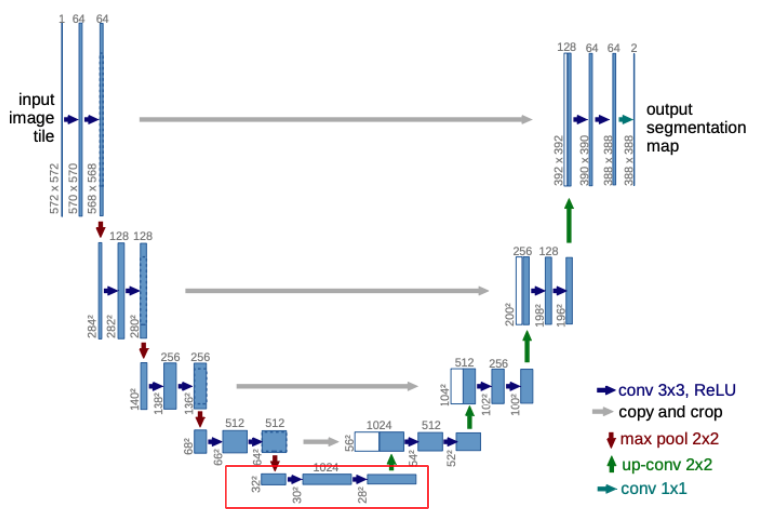
After the contracting path, it goes through another double_conv layers which will be fed into the expansive path as the input.

Expansive Path

U-Net

After going through the contracting path and the bottle layer, it enters the expansive path. The expansive path utilizes transpose convolution which performs upsampling, increasing the resolution of the input. The 2 x 2 transpose convolution halves the number of channel dimension and doubles the spatial dimension.

For better localization, high resolution features from the contracting path are concatenated with the upsampled output to provide a more precise output based on this information.

A more intuitive interpretation for this concatenation is that at each depth of the network, the level of abstraction differs. For example, the very first output in the contracting path provides low-level semantics of the given image such as curves and edges. Now, the corresponding feature map in the expansive path (top-right) is nearly close to the final prediction which requires dense and sophisticated prediction. Also, the input of the top-right feature map in the expansive path has already gone through the previous expansive pathways with the concatenations of higher-level context information from the contracting path. Therefore, the expansive network gradually turns higher-level context information into more precise and dense prediction as it goes up.

Skip Connection

U-Net

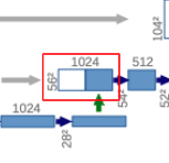
Here I provide a more detailed explanation of skip connection or concatenation. In the original paper, the feature map from the contracting path is cropped to match the spatial dimension of the feature map from the expansive path. Don’t get confused that in the figure above, the blue-colored is the one from the expansive path after transpose convolution and the white-colored is the concatenated feature map from the contracting path.

Final Layer

U-Net

After going through contracting path, bottleneck layer, and expansive path, we need to address our ultimal goal: semantic segmentation. The semantic segmentation assigns a class label to each pixel value.

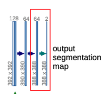
In U-Net, 1 x 1 convolutional layer (n filters) is attached to the final output of the expansive path where n is the number of classes for our task. For example, if we have dog, cat and sheep classes, the final output segmentation map will have 3 channels. We can apply channel-wise softmax to determine the final prediction of the class label for a specific pixel.

Overlap-tile Strategy

U-Net

As you might’ve noticed, the input image and the final output have different image resolution. Since the double_conv used 0 padding, the resolution decreases after each convolution layer. Consequently, the input image has 572 x 572 resolution while the final prediction has 388 x 388 resolution in the example above. Hence, the original U-Net produces a slightly condensed segmentation map.

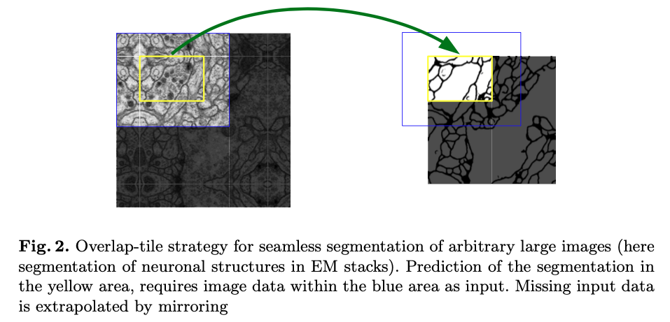
U-Net accpets any arbitrary sized input image. For better utilization of GPU, the author used overlap-tile strategy which divides the input image into k x k tiles. Each tile is then fed into the U-Net model. This is it says input image tile instead of input image in the architecture figure.

Since the input and the output have different resolutions, the missing context is extrapolated by mirroring the input image as you can see in the figure above.

Network Architecture

Here’s a summary of the overall network architecture (although most of them already mentioned above).

Contracting path

double_conv which consists of two 3x3 convolutions (unpadded), each followed by ReLU and a 2x2 max pooling with stride 2 for downsampling. At each downsampling step, the feature channels get doubled.

Expansive Path

double_conv is applied in the expansive path but the feature channels get halved. Instead of max pooling, 2 x 2 transpose convolution is applied, each followed by ReLU.

Final Layer

1 x 1 convolution (n filters) is applied where n denotes the number of classes for our task.

Data Augmentation

For better performance with a very few images, the author used heavy data augmentation to provide diverse training data distribution. As this paper originally aimed for microscopical images, U-Net used shift and rotation, elastic deformations, gray value variations, smooth deformations using random displacement vectors on a coarse 3 by 3 grid. Drop-out layers are applied at the end of the contracting path.

Experiments

Semantic Segmentation

PyTorch Implementation

model.py

import torch
import torch.nn as nn
from utils import crop_img, concat_imgs_crop

def double_conv(in_channel, out_channel):
    conv = nn.Sequential(
        nn.Conv2d(in_channel, out_channel, kernel_size=3, padding=0),
        nn.ReLU(inplace=True),
        nn.Conv2d(out_channel, out_channel, kernel_size=3, padding=0),
        nn.ReLU(inplace=True)
    )

    return conv


def trans_conv(in_channel, out_channel):
    return nn.ConvTranspose2d(in_channel, out_channel, kernel_size=2, stride=2)


class UNet(nn.Module):
    def __init__(self, in_channels=3, n_classes=10):
        super(UNet, self).__init__()
        self.n_classes = n_classes

        self.max_pool = nn.MaxPool2d(kernel_size=2, stride=2)

        # Encoder - Contracting Path
        self.down_conv_1 = double_conv(in_channels, 64)
        self.down_conv_2 = double_conv(64, 128)
        self.down_conv_3 = double_conv(128, 256)
        self.down_conv_4 = double_conv(256, 512)
        self.down_conv_5 = double_conv(512, 1024) # bottleneck

        # Decoder - Expansive Path
        self.up_conv_1 = double_conv(1024, 512)
        self.up_conv_2 = double_conv(512, 256)
        self.up_conv_3 = double_conv(256, 128)
        self.up_conv_4 = double_conv(128, 64)

        # Final Layer
        self.final_layer = nn.Conv2d(64, n_classes, kernel_size=1)

    def forward(self, img):
        '''
        img: (B, C, H, W)
        '''

        # Encoder - Contracting Path
        d1 = self.down_conv_1(img) # concat
        d2 = self.down_conv_2(self.max_pool(d1)) # concat
        d3 = self.down_conv_3(self.max_pool(d2)) # concat
        d4 = self.down_conv_4(self.max_pool(d3)) # concat
        d5 = self.down_conv_5(self.max_pool(d4)) # bottleneck

        # Decoder - Expansive Path
        u4 = trans_conv(1024, 512)(d5)
        u4 = concat_imgs_crop(d4, u4)

        u3 = trans_conv(512, 256)(self.up_conv_1(u4))
        u3 = concat_imgs_crop(d3, u3)

        u2 = trans_conv(256, 128)(self.up_conv_2(u3))
        u2 = concat_imgs_crop(d2, u2)

        u1 = trans_conv(128, 64)(self.up_conv_3(u2))
        u1 = concat_imgs_crop(d1, u1)

        out = self.up_conv_4(u1)

        # Final Layer
        out = self.final_layer(out)
        print(out.shape)

        return out


if __name__ == '__main__':
    img = torch.rand(1, 3, 572, 572)
    model = UNet(in_channels=3, n_classes=10)
    model(img)

utils.py

import torch
import torchvision
import torchvision.transforms.functional as TF

def crop_img(original, target):
    '''
    :param original: (B, C, H, W)
    :param target: (B, C, H, W)
    '''
    target_size = target.size()[2]
    original_size = original.size()[2]

    delta = original_size - target_size

    delta_1 = delta // 2
    delta_2 = delta - delta_1

    return original[:, :, delta_1:original_size-delta_2, delta_1:original_size-delta_2]


def concat_imgs_crop(down_tensor, up_tensor):
    '''
    Concatenate 'down_tensor' and 'up_tensor' along dim-1.
    'down_tensor' must be cropped to match the resolution of 'up_tensor'

    :param down_tensor (tensor): from contracting pathway. Shape: (B, C, H, W)
    :param up_tensor (tensor): from expansive pathway. Shape: (B, C, H, W)

    :return cropped tensor
    '''
    cropped_down_tensor = crop_img(down_tensor, up_tensor)
    return torch.cat([cropped_down_tensor, up_tensor], dim=1) # channel-wise concat

Github

Here is the full implementation with dataset.py, train.py, etc.

https://github.com/JasonLee-cp/deep-learning-papers/tree/master/u_net

References

[1] https://arxiv.org/abs/1505.04597

[2] https://medium.com/@msmapark2/u-net-%EB%85%BC%EB%AC%B8-%EB%A6%AC%EB%B7%B0-u-net-convolutional-networks-for-biomedical-image-segmentation-456d6901b28a

[3] https://towardsdatascience.com/unet-line-by-line-explanation-9b191c76baf5