Introduction
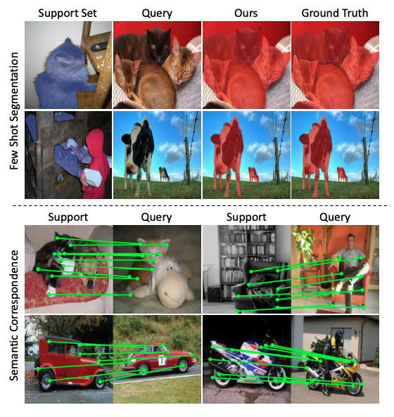
Semantic segmentation task is of an extreme importance due to its many applications such as medical image analysis, self-driving, and video editing. However, it takes great time and human effort to manually annotate the training datasets which is very ineffective. Therefore, few-shot segmentation task has been increasingly important as it requires only a number of support samples to predict the segmentation mask for the query image. This significantly removes the burdens of time-consuming manual annotation.
Many methods for few-shot segmentation have been proposed and most of them follow a learning-to-learn design to avoid the overfitting resulting from the small training dataset. Since the prediction on the query image should be “conditioned” on the support images, the essential task of few-shot segmentation is how to effectively utilize support samples. Many works tried to utilize a prototype from support samples but these approaches disregard pixel-wise relationships between the support and query samples.
The paper suggests that few-shot segmentation task can be framed as semantic correspondence task which finds pixel-wise correspondences between semantically similar images. Dense pixel correspondences possess some challenges such as large intra-class appearance and geometric variations. The latest works focused on cost aggregation stage to mitigate that issue.
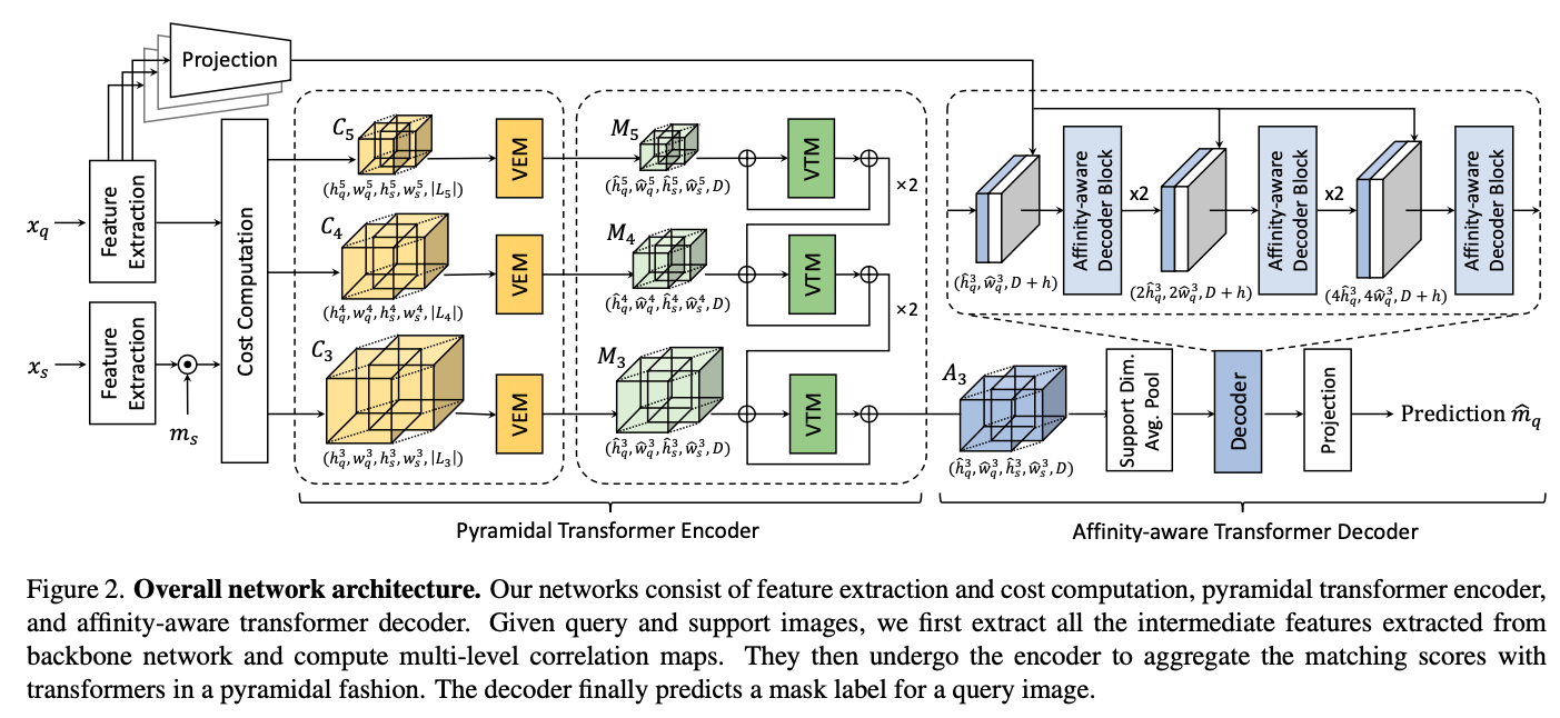
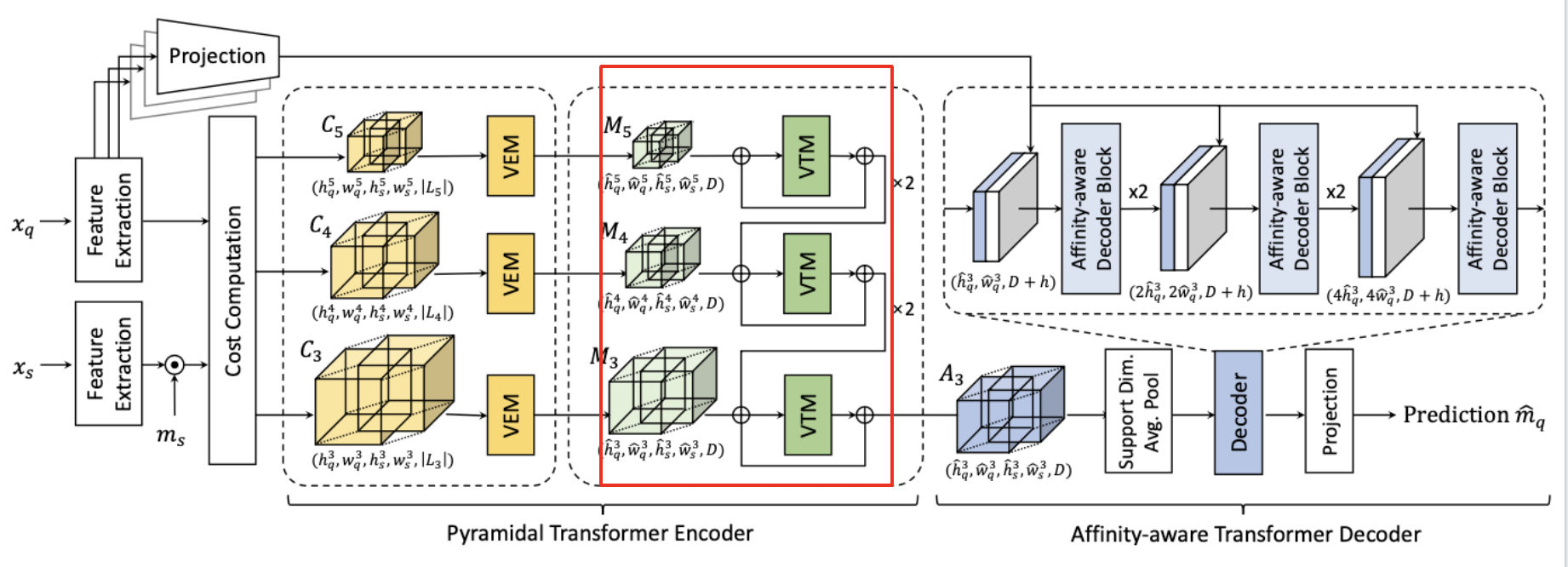
In this paper, a cost aggregation network called Volumetric Aggregation with Transformers (VAT) is proposed which uses both convolutions and transformers to extract high-dimensional correlation maps between the query and support samples. In the bird’s eye view, VAT consists of three modules which we will cover one-by-one soon.
Volumetric Embedding Module (VME)
Volumetric Transformer Module (VTM)
Affinity-aware Decoder
Overall Network Architecture
Problem Formulation
The goal of few-shot segmentation is to produce the segmentation mask of an object of unseen class from a query image, but only with a few annotated support samples. In order to mitigate the overfitting problem casued by the small dataset, the common protocol called episodic training is used.
Let’s denote traning and test set as $\mathcal{D_{train}}$ and $\mathcal{D}_{test}$, respectively where object classes of the sets do not overlap.
Under $K$-shot setting, multiple episodes from both sets. Each episode consists of a support set \(\mathcal{S}\) and query sample \(\mathcal{Q}\).
\[\mathcal{S}=\{(x_s^k, m_s^k)\}\_{k=1}^K\]where \((x_s^k, m_s^k)\) is \(k-th\) support image and its corresponding segmentation mask pair.
and eof a query sample
\[\mathcal{Q} = (x_q, m_q)\]where \(x_q\) and \(m_q\) are a query image and mask, respectively.
Then, the model takes a sampled episode from \(\mathcal{D}\_{train}\) during training and learns a mapping from \(\mathcal{S}\) and \(x_q\) to a prediction \(m_q\).
During inference time, the model predicts \(\hat{m}_q\) for randomly sampled \(\mathcal{S}\) and \(x_q\) from \(\mathcal{D}\_{test}\).
VAT Overview
The essential part of few-shot segmentation is how to effectiely utilize a few support samples for a query image. To achieve this, Volumetric Aggregation with Transformers (VAT) effectively intergrates information in all pixel-wise matching costs between query and support samples with transformers.
To mitigate the high computational cost of transformers, VAT proposes volume embedding module to reduce the number of tokens while inserting the inherent inductive biases fo convolutional layers. Also, Volume Transformer Module (VTM) based on swin transformer is used to reduce the computational complexity. VAT is an encoder-decoder architecture.
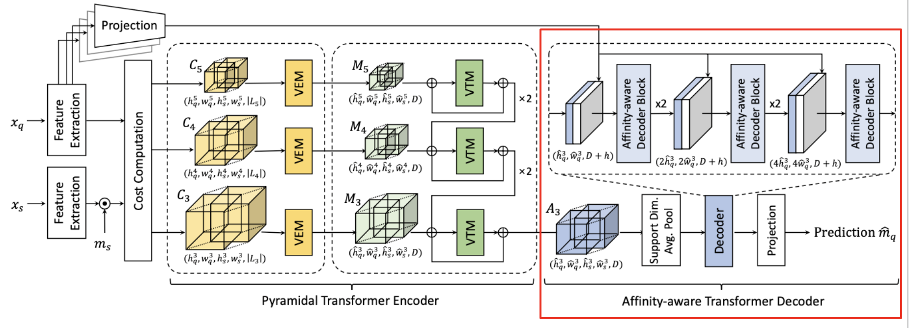
The encoder is designed in a pyramidal manner to make the output from coarser level cost aggregation to guide the finer level. The decoder utilizes appearance affinity module to resolve the ambiguities presented in the raw correlation map.
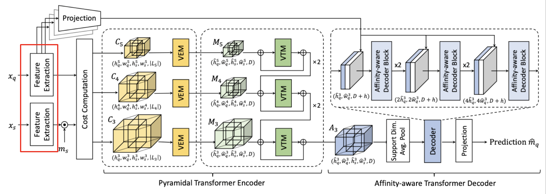
Feature Extraction and Cost Computation
In order to compute the initial cost between the query and the support samples, we extract the multi-level features by CNNs.
Query and support images are denoted as \(x_q\) and \(x_s\). From them, we produce a sequence of \(L\) feature maps \(\{ (F_q^l, F_s^l) \}_{l=1}^L\) where \(F_q^l\) and \(F_s^l\) denote query and support feature maps at \(l-th\) level, respectively.
With the support mask \(m_s\), we encode the segmentation information and filter out the background information. Then, we obtain a masked support feature such that
\[\hat{F}\_s^l = F_s^l \odot \psi^l(m_s)\]where \(\odot\) denotes element-wise product and \(\psi^l(\cdot)\) denotes a function that resizes the given tensor followed by expansion along channel dimension of \(l-th\) layer.
After obtaining the pair of feature maps from the query and the sample, \(F_q^l\) and \(F_s^l\), we then compute the correlation map by the inner product between the L2 normalized features,
\[\mathcal{C}^l(i,j) = ReLU \left( \frac{F_q^l(i) \cdot \hat{F}\_s^l(j)}{\lVert F_q^l(i)\rVert \lVert \hat{F}\_s^l (j) \rVert} \right)\]where \(i\) and \(j\) denote 2D spatial positions of feature maps.
Then, we collect the correlation maps from all the intermediate features of same spatial size. Next, we concatenate them to obtain a hypercorrelation
\[\mathcal{C}_p = \{\mathcal{C}^l \}_{l \in \mathcal{L})p},\ \ \mathbb{R}^{h_q \times w_q \times h_s \times \lvert \mathcal{L}\_p \rvert}\]where \(h_q, w_q\) and \(h_s, w_s\) are height and width of feature maps of query and support samples, respectively. \(\mathcal{L}_p\) is subset of CNN layer indices \(\{ 1,...,L \}\) at some pyramid layer \(p\) with the identical spatial size correlation maps.
Pyramidal Transformer Encoder
Next, we’ll talk about Volumne Embedding Module (VEM) and Volumetric Transformer Module (VTM)
Volume Embedding Module (VEM)
Now we have the hypercorrelation. However, we cannot just aggregate along all the spatial dimensions as there’re too many tokens, resulting in extremely heavy computations.
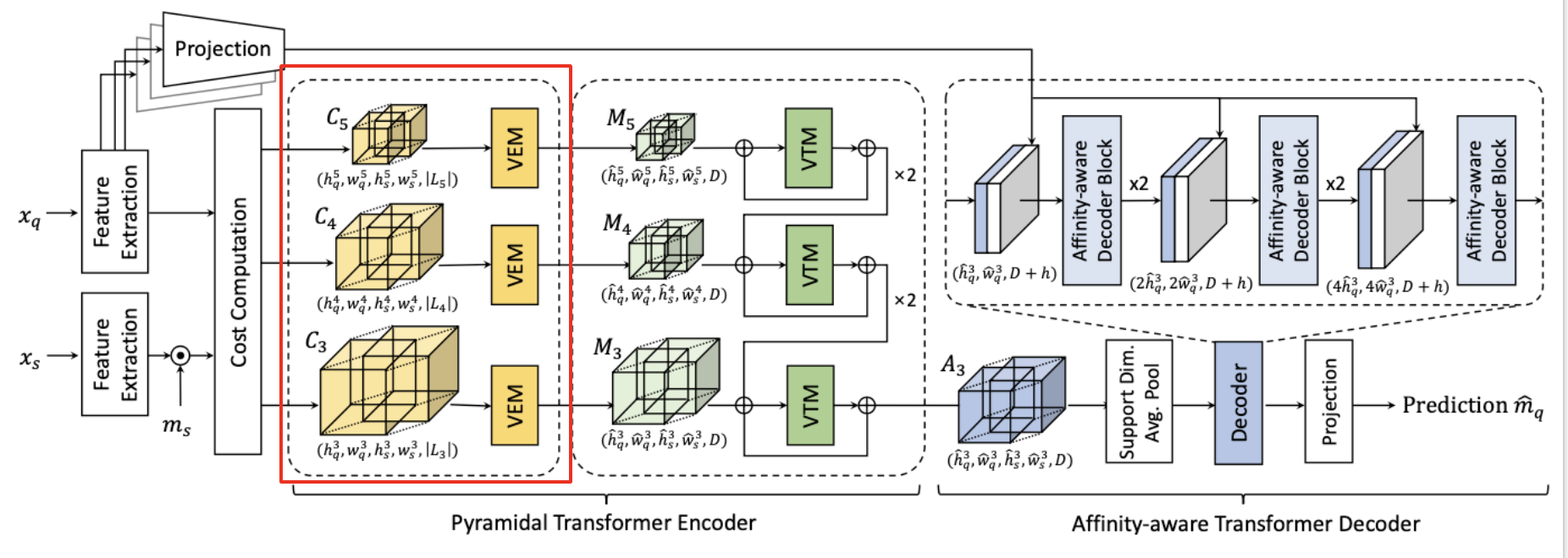
To mitigate this issue, Volume Embedding Module (VEM) is proposed to reduce the computational complexity by decreasing the number of tokens and injecting inductive biases of convolutional layers. This strategy enables the subsequent transformer model to better learn interactions among the hypercorrelations.
Specifically, we apply 4D spatial max-pooling, overlapping 4D convolutions, ReLU, and Group Normalization (GN). We project the multi-level similarity vector at each 4D position.
Given a vector size of \(\lvert \mathcal{L}_p \rvert\), we project it to a arbitrary fixed dimension \(D\).
Considering receptive fields of VEM as 4D window size, we construct a tensor
\[\mathcal{M} \in \mathbb{R}^{\hat{h}\_q \times \hat{w}\_q \times \hat{h}\_s \times \hat{w}\_s \times D}\]where \(\hat{h}\) and \(\hat{w}\) are the processed sizes.
The overall process can be formulated as
\[\mathcal{M}\_p = VEM(\mathcal{C}\_p)\]Volumetric Transformer Module (VTM)
Even though the computational complexity is mitigated by VEM, applying self-attention is still challenging with its quadratic complexity. VAT thus utilizes Volumetric Transformer Module (VTM) based on powerful swin transformer which utilizes local window attention, reducing time complexity significantly. More details on swin transformer could be found on my post. It’s proven that neighboring pixels are likely to have similar correspondences. Thus, calculating self-attnetion in local windows go well along with this nature. Also, cross-window interaction of swin transformer architecture helsp to find reliable correspondences. The use of 4D convlution lacks an ability to consider pixel-wise interactions due to the fixed kernels during convolution while transformers explore the pixel-wise global interactions.
In VTM, we first partition query and support spatial dimensions of \(\mathcal{M}_p\) into non-overlapping sub-hypercorrelations
\[\mathcal{M}'\_p \in \mathbb{R}^{n \times n \times n \times n \times D}\]Then, we calculate self-attention within each partitioned sub-hypercorrelation. Then, we shift the windows by displcement of \((\lfloor \frac{n}{2}\rfloor, \lfloor \frac{n}{2}\rfloor, \lfloor \frac{n}{2}\rfloor, \lfloor \frac{n}{2}\rfloor)\) pixels from the partitioned windows. We then perform self-attention within the newly created windows.
Next, we apply cyclic shift like the original swin transformer to its original form.
VAT also uses relative position bias like swin transformer. Other components of swin transformer remain unchanged.
Moreoever, to make the learning more stable and to prevent bad parameter initializations, we make the network to learn the residual matching scores..
The overall process can be formulated as,
\[\mathcal{A}\_p = VTM(\mathcal{M}\_p) = \mathcal{\mathcal{M}\_p} + \mathcal{M}\_p\]where \(\mathcal{T}\) denotes transformer module.
Pyramidal Processing
It’s shown that utilizing multi-level features shows significant performance gain. Hence, VAT utilizes the coarse-to-fine approach through a pyramidal hypercorrelation where the finer level aggregated correlation map \(\mathcal{A}_p\) is “guided” by the aggregated correlation map of previous levels \(\mathcal{A}\_{p+1}\).
Specifically, the aggreagated correlation map \(\mathcal{A}\_{p+1}\) is upsampled, denoted as \(up(\mathcal{A}\_{p+1})\) and added to next level’s correlation map \(\mathcal{A}_p\) as a guidance.
This process is applied until the finest level before the decoder.
The pyramidal process can be formulated as,
\[\mathcal{A}\_p = VTM(\mathcal{M}\_p + up(\mathcal{A}\_{p+1}))\]Affinity-Aware Transformer Decoder
As done in Cost Aggregation Transformers (CATs), VAT also utilizes appearance embedding extracted from query feature maps for more accurate correspondence. The appearance affinity helps to filter out the incorrect matching scores.
For the decoder part, we first average over support dimensions of \(\mathcal{A}_p\) which is concatenated with appearance embedding. Then, it’s processed by swin transformer followed by bilinear interpolation. The overall process can be formulated as,
\[\hat{\mathcal{A}}' = Decoder([\hat{\mathcal{A}}, \mathcal{P}(F_q)])\]where \(\hat{A} \in \mathbb{R}^{\hat{h}_q \times \hat{w}_q \times D}\) is extracted by average-pooling in its support spatial dimensions. \(\mathcal{P}(\cdot)\) denotes linear projection \(\mathcal{P}(F_q) \in \mathbb{R}^{\hat{h}_q \times \hat{w}_q \times h}\). \(\hat{A}\) is bilinear upsampled and goes through the above equation until the projection head which predicts the final mask \(\hat{m}_q\).
\(K\)-Shot Setting
When \(K>1\), given \(K\) pairs of support image and mask and a query image, the model forward-passes \(K\) times to obtain \(K\) predictions. Then, the model finds the maximum number of predictions labelled as foreground across all the spatial locations (hard voting). The output is considered as foreground if the output divided by \(k\) is above the given threshold and otherwise background.
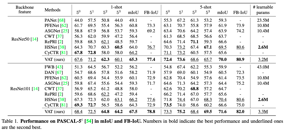
Experiments
\[\]References

