Introduction
Hello there! welcome to the new episode: Vision Transformer which you might’ve heard before. I highly recommend you to go through the breakthrough paper Attention is all you need which is a foundation of ViT. Alternatively, Illustrated Transformer is a wonderful resource to get a solid grasp on transformer. After you go over how transformer works, ViT becomes very easy to understand.
The transformer architecture has swept away natural language processing (NLP) field with its brilliant attention-mechanism and computational efficiency and scalability. It has become the de-facto standard ever since. However, transformer was not yet fully mature in vision tasks such as image classification, object detection, and segmentation at the time when ViT was published, 2020. As one could imagine, there have been many proposed ways of integrating transformer into vision tasks such as partially replacing convolutional layers or using transformer in conjunction with CNN. Meanwhile, ViT suggests fully transformer-based architecture for image classification tasks without using CNN (although one CNN layer is used in implementation for efficiency which we’ll talk about shortly).
Self-Attention
Let’s briefly review attention mechanism. The core idea of attention mechanism is that each word would have some sort of relations with other words in a sentence. For example, in the sentence “Jason didn’t go to school because he was too tired”, the word “he” cannot be entirely interpreted without “attending” to the word “Jason”. This is obviously true as we know the word “he” is a pronoun referring to the name “Jason”. Also, “tired” is more related or more “attends” to “he” or “Jason” than “school”. This is why we use attention mechanism: to untangle the attention of a word to other words in a sentence.
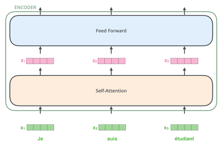
Now let’s see how attention is calculated. Below are great visualizations from Illustrated Transformer.
Below is the overview of transformer architecture. Each word (token) is embedded and fed into the transformer. After going through self-attention, it’s fed into the feed-forward layer.
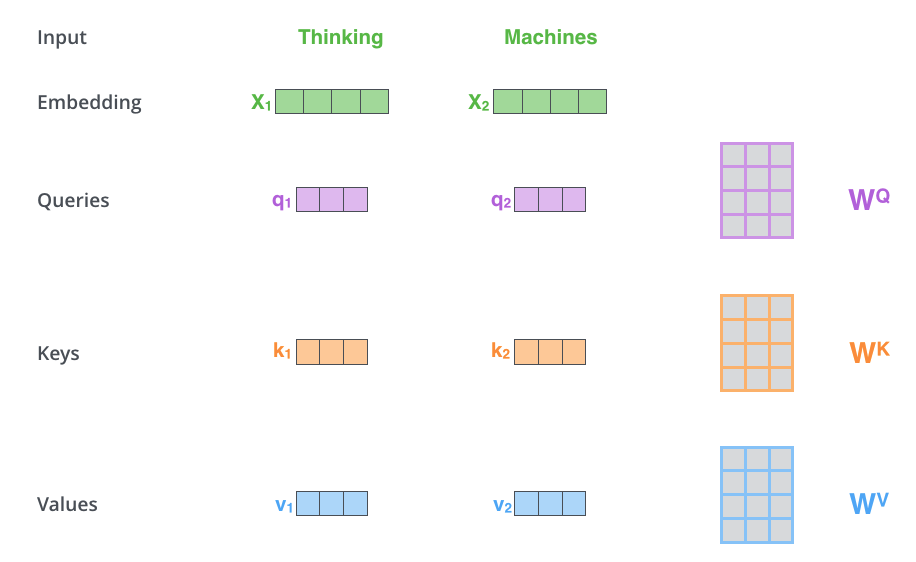
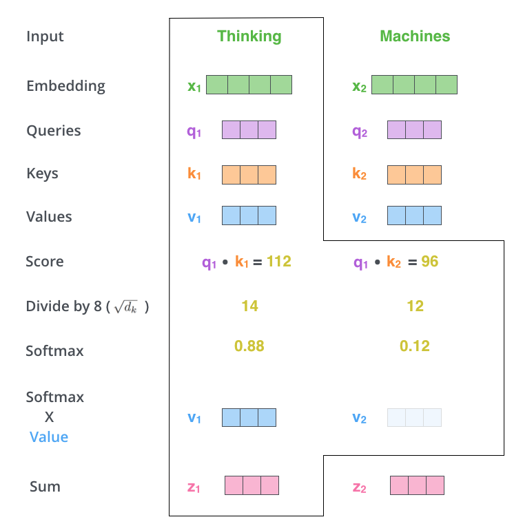
Now, how is self-attention calculated?
We create the query, key, and value vectors for each embedded vector. Then, we multiply query and key to get score. We normalize the score by \(\sqrt{d_k}\) where \(d_k\) is the embedding dimension (64 in this case). Next, we apply softmax function to obtain the attention for each token. Finally, we get the weight sum by multiplying these outputs from softmax with the value vector.
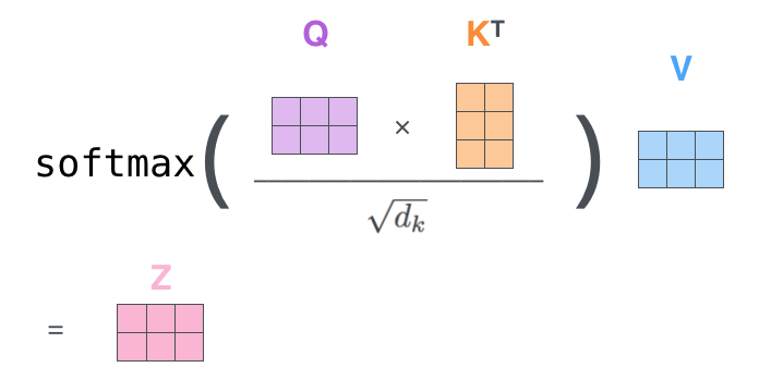
We can do self-attention for every token in one-shot using matrix multiplication.
Multi-head Attention
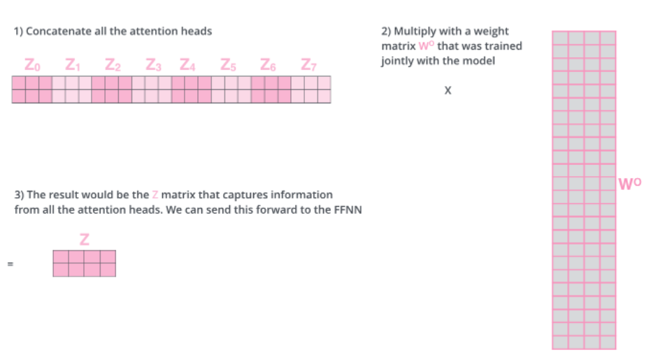
So far, we had only one atttention head. Instead of 1, we can use multiple heads for attention. This is very simple. Just perform the above self-attention for individual head and concatenate them. Then, multiply with a weight matrix to obtain the single \(Z\) vector.
ViT Architecture
Great! Now we know how transformer works. But how do we apply transformer to images?
One naive application of transformer is to treat each pixel as a token so that each pixel attends to every other pixel. However, with the quadratic cost in the number of pixels, this is unrealistic.
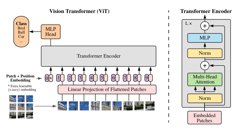
Instead, ViT splits an image into fixed-size patches. If an image is H x W, there’re 3 channels, and each patch has P x P size, then each patch has \(C \cdot P^2\) pixels and there are total of \(\frac{H}{P} \cdot \frac{W}{P} = \frac{HW}{P^2}\) patches for an image.
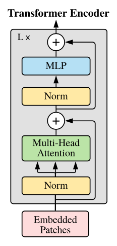
Then, as shown in the right in the figure, embedded patches go through the transformer encoder which consists of layer norm, multi-head attention, and MLP layers with dropout after multi-head attention and skip connection.
It’s quite simple right? We’re done! The core idea of ViT is to treat each patch as a token and feed the those patches into the transformer encoder. The author mentioned that ViT follows pretty much the same original transformer architecture. This transformer encoder is repeated L times. Lastly, the resulting vectors go through the classification head for classification.
With this overall architecture in mind, let’s look at some details of the architecture with PyTorch implementation.
Patch Embedding
The patch embedding block consists of flattening, linear projection, class tokens, and position embeddings. I believe it’s the best to understand with codes. Below is the full patch embedding code and each module is followed with description.
1
2
3
4
5
6
7
8
9
10
11
12
13
14
15
16
17
18
19
20
21
22
23
24
25
26
27
28
29
30
31
32
33
34
35
36
37
38
39
40
41
42
43
44
45
import torch
import torch.nn as nn
import torch.nn.functional as F
from einops import rearrange, reduce, repeat
from einops.layers.torch import Rearrange, Reduce

class PatchEmbedding(nn.Module):
    def __init__(self, in_channels=3, patch_size=16, emb_dim=768, img_size=224):
        super().__init__()
        self.patch_size = 16
        self.n_patches = (img_size ** 2) // (patch_size ** 2)

        # [1] Project Method 1
        self.img2token = Rearrange('b c (h p1) (w p2) -> b (h w) (c p1 p2)', p1=patch_size, p2=patch_size)
        self.linear_projection = nn.Linear(in_channels * (patch_size ** 2), emb_dim)

        # [1] Project Method 2 using Conv2d
        self.projection = nn.Sequential(
            nn.Conv2d(in_channels, emb_dim, patch_size, stride=patch_size),
            Rearrange('b e h w -> b (h w) e')
        )

        # [2] Class Token - from BERT
        self.cls_token = nn.Parameter(torch.randn(1, 1, emb_dim))

        # [3] Position Embedding
        self.position_embedding = nn.Parameter(
            torch.randn(self.n_patches + 1, emb_dim)
        )


    def forward(self, x):
        B = x.shape[0]

        # [1] Tokenize & Linear Projection
        x = self.projection(x) # (B, n, e)

        # [2] Prepend class tokens
        cls_tokens = repeat(self.cls_token, '() n e -> b n e', b=B)
        x = torch.cat([cls_tokens, x], dim=1) # (B, n+1, e)

        # [3] Position Embedding
        x += self.position_embedding # (B, n+1, e)

        return x
Flatten & Linear Projection
Suppose we have an image with H x W resolution with C channels. We first flatten the image it to N x (C x P x P) where P is a patch size (16) and N is the number of patches HW/P^2. Then, linearly project these patches into D dimensions (768) with a trainable linear projection. We can do this in two ways: (1) vanilla projection and (2) using CNN. Let’s look at the implementation (using einops).
Vanilla Projection
1
2
3
# [1] Project Method 1
self.img2token = Rearrange('b c (h p1) (w p2) -> b (h w) (c p1 p2)', p1=patch_size, p2=patch_size)
self.linear_projection = nn.Linear(in_channels * (patch_size ** 2), emb_dim)
CNN Projection
1
2
3
4
5
# [1] Project Method 2 using Conv2d
self.projection = nn.Sequential(
    nn.Conv2d(in_channels, emb_dim, patch_size, stride=patch_size),
    Rearrange('b e h w -> b (h w) e')
)
Class Token
We prepend a learnable embedding, class token, to the sequence of embedded patches, whose “state” at the output of the encoder serves as the image representation.
1
2
# [2] Class Token - from BERT
self.cls_token = nn.Parameter(torch.randn(1, 1, emb_dim))
Position Embedding
Since plain transformer architecture does not contain information about the relative ordering of the patches, position embeddings are added to retain positional information. We use standard learnable 1D position embeddings.
1
2
3
4
# [3] Position Embedding
self.position_embedding = nn.Parameter(
    torch.randn(self.n_patches + 1, emb_dim)
)
Transformer Encoder
The transformer encoder consists of two blocks as shown in the figure above. Let’s look at the implementation in a top-down fashion. The number of repeated transformer encoders is 12.
Imports
1
2
3
4
import torch
import torch.nn as nn
import torch.nn.functional as F
from einops import reduce, rearrange, repeat
Encoder
1
2
3
4
5
6
7
class Encoder(nn.Sequential):
    def __init__(self, depth=12, emb_dim=768, n_heads=8, attn_drop=0.,
                 drop_path=0., expansion=4):
        super().__init__(
            *[EncoderBlock(emb_dim, n_heads, attn_drop, drop_path, expansion)
              for _ in range(depth)]
        )
Encoder Block
1
2
3
4
5
6
7
8
9
10
11
12
13
14
15
16
17
18
19
20
21
22
23
24
25
26
class EncoderBlock(nn.Module):
    def __init__(self, emb_dim=768, n_heads=8, attn_drop=0.,
                 drop_path=0., expansion=4):
        super().__init__()
        self.block1 = nn.Sequential(
            nn.LayerNorm(emb_dim),
            MultiHeadAttention(emb_dim, n_heads, attn_drop),
            nn.Dropout(drop_path)
        )

        self.block2 = nn.Sequential(
            nn.LayerNorm(emb_dim),
            MLP(emb_dim, expansion, drop_path),
            nn.Dropout(drop_path)
        )

    def forward(self, x):
        skip1 = x
        x = self.block1(x)
        x += skip1

        skip2 = x
        x = self.block2(x)
        x += skip2

        return x
Multi-head Attention
It’s simpler (maybe more complicated) to use matrix multiplication which could handle the query, key, value vectors in one-shot. One thing to note that is d_h is the embedded dimension for each head. The original embedding dimension was 768. The paper used d_h as \(\frac{D}{\text{h}}\) where \(h\) is the number of heads (8), and \(D\) is the original embedding dimension (768). Hence, the embedding dimension for each head is 96. It might be a bit tricky to understand but try to write down the dimensions on a piece of paper and follow through.
1
2
3
4
5
6
7
8
9
10
11
12
13
14
15
16
17
18
19
20
21
22
23
24
25
class MultiHeadAttention(nn.Module):
    def __init__(self, emb_dim=768, n_heads=8, attn_drop=0.):
        super().__init__()
        self.emb_dim = emb_dim
        self.n_heads = n_heads

        self.qkv = nn.Linear(emb_dim, emb_dim * 3)
        self.attn_drop = nn.Dropout(attn_drop)
        self.projection = nn.Linear(emb_dim, emb_dim)

    def forward(self, x):
        qkv = self.qkv(x)
        qkv = rearrange(qkv, "b n (h d qkv) -> qkv b h n d", h=self.n_heads, qkv=3)
        q, k, v = qkv[0], qkv[1], qkv[2] # each (b, h, n, d_h)

        d_h = (self.emb_dim / self.n_heads) ** (0.5)
        attention = torch.einsum('bhqd, bhkd -> bhqk', q, k) # (b, h, n, n)
        attention = F.softmax(attention, dim=-1) / d_h
        attention = self.attn_drop(attention) # (b, h, n, n)

        out = torch.einsum('bhqk, bhvd -> bhqd', attention, v) # (b, h, n, d_h)
        out = rearrange(out, "b h n d_h -> b n (h d_h)") # (b, n, d)
        out = self.projection(out) # (b, n, emb_dim)

        return out
MLP
The MLP layer contains two layers with a GELU non-linearity and dropout.
1
2
3
4
5
6
7
8
class MLP(nn.Sequential):
    def __init__(self, emb_dim, expansion=4, drop_path=0.):
        super().__init__(
            nn.Linear(emb_dim, emb_dim * expansion),
            nn.GELU(),
            nn.Dropout(drop_path),
            nn.Linear(emb_dim * expansion, emb_dim)
        )
Classification Head
Lastly, the resulting vectors go through the classification head to give us the final prediction for image classification.
1
2
3
4
5
6
7
8
9
10
11
import torch.nn as nn
from einops.layers.torch import Reduce

class ClassificationHead(nn.Sequential):
    def __init__(self, emb_dim=768, n_classes=10):
        super().__init__(
            Reduce('b n e -> b e', reduction='mean'),
            nn.LayerNorm(emb_dim),
            nn.Linear(emb_dim, n_classes)
        )
ViT: Putting all together
1
2
3
4
5
6
7
8
9
10
11
12
13
14
15
16
17
18
19
20
21
22
23
24
25
26
27
28
29
30
31
32
33
34
35
36
37
38
39
40
41
42
43
import torch
import torch.nn as nn

from patch_embedding import PatchEmbedding
from encoder import Encoder
from classification_head import ClassificationHead

from torchsummary import summary

class ViT(nn.Module):
    def __init__(self,
                 in_channels=3,
                 patch_size=16,
                 n_heads=8,
                 emb_dim=768,
                 attn_drop=0.,
                 drop_path=0.,
                 expansion=4,
                 img_size=224,
                 depth=12,
                 n_classes=10,
                 ):
        super().__init__()

        self.patch_embedding = PatchEmbedding(in_channels, patch_size, emb_dim, img_size)
        self.encoder = Encoder(depth, emb_dim, n_heads, attn_drop, drop_path, expansion)
        self.classification_head = ClassificationHead(emb_dim, n_classes)

    def forward(self, x):
        x = self.patch_embedding(x)
        x = self.encoder(x)
        x = self.classification_head(x)
        return x

dummy = torch.randn(4, 3, 224, 224)
vit = ViT()
out = vit(dummy)
print("Output shape: {}".format(out.shape))

"""
Output shape: torch.Size([4, 10])
"""
Inductive Bias
Great job! We’ve dived deep into how ViT works. However, here comes a very important concept, inductive bias, to further understand ViT. You might’ve heard that ViT requires extensive data to have a good performance. When trained on mid-sized datasets such as ImageNet without strong regularization, ViT yields accuracy worse than CNN models. Why does this happen? The most plausible reason is that the transformers lack some of the inductibe biases inherent to CNNs such as translation invariance and locality.
Inductive bias is any belief or assumption we have about the unseen data. Let’s take an example. Suppose we want to predict a housing price based on house size, number of floors, and number of bedrooms. One possible way of modeling architecture is to have a complex model with 30 billion parameters. On the other hand, we can utilize our humans’ common sense that those three criteria are somehow linearly correlated to the house price. This is exactly what the inductive bias is about. We made an assumption that house price is linearly correlated to those criteria. Then, we can more effectively design and train our model for this specific “house price prediction” task without consuming heavy computational resources. The first model with tons of parameters would require extensive dataset to figure out the “linear relationship” since it literally starts training from scratch.
Inductive bias can be categorized into two different groups: relational inductive bias and non-relational inductive bias.
Relational Inductive Bias
Relational inductive bias is a type of inductive bias. Relational inductive bias representes the relationships between entities in the network.
The convolutional neural network, CNN, uses kernels or filters which capture local relationships between the entities in the kernel. Hence, CNN has locality relational inductive bias. Also, the entities(pixels) in CNN are locally grouped so CNN has weak global relationships while the plain FCN densely connects the entities. Consequently, CNN is good at capturing features of an image which is suitable for image classification. With this characteristic, CNN has translation invariance relational inductive bias which means translation of a cat in an image is still classified as a cat. Also, CNN has translation equivariance relational inductive bias since if you feed input with different positions, the output feature map will be focusing on the specific position of the objects. This translational equivariance property is converted into translation invariance by the last layers for classification. Lastly, CNN has 2D neighborhood structure.
On the other hand, transformer architecture has a weak image-specific inductive bias. In ViT, only MLP are local and translation equivariance while the self-attention is global. The two-dimensional neighborhood structure is only used in the beginning where the image is cut into patches and at fine-tuning time for adjusting the position embeddings.
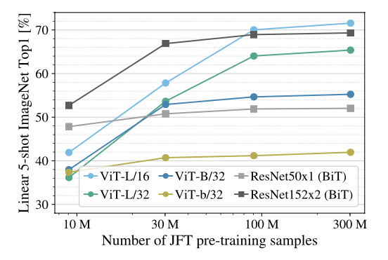
With this weak inductive bias, transformer needs extensive dataset since it has to learn about the 2D positions of patches and all spatial relations between the patches from scratch. Although ViT shows suboptimal performances with small or mid-sized (worse than CNN), it outperforms CNN-based models with large dataset.
Model Variants
Performances
The above figure shows the comparison between ViT and other models. Notice that ViT shows better performance when trained on the huge dataset JFT-300M while taking substantially less time.
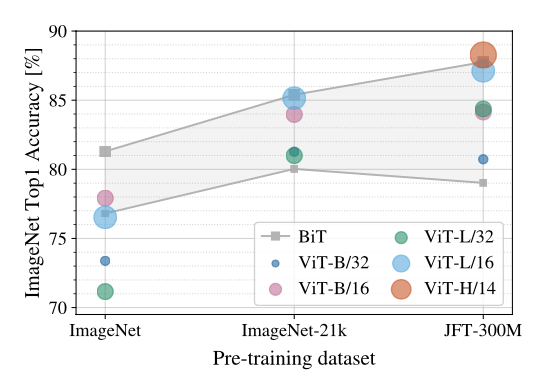
The above figure shows the performances trained on different datasets. Notice that BiT ResNets perform better than ViT models for small dataset (ImageNet) but ViT outperforms when trained on larger datasets
The above figure shows Few-shot evaluation on ImageNet with different pre-training sizes. ResNet outperforms ViT with smaller pre-training datasets but plateau sooner than ViT. ViT shows better performances with larger pre-training.
Source Code
References
[1] https://arxiv.org/abs/2010.11929
[2] https://github.com/FrancescoSaverioZuppichini/ViT
[3] https://jalammar.github.io/illustrated-transformer/

